——–

——–
Table of Contents

1. General Safety Requirements ……………………………….. 1
   
2. Safety Terms and Symbols ……………………………………. 2
   
3. Quick Start …………… 4
   

Introduction to the Structure of the Oscilloscope …. 4

Front Panel ………… 4

Rear Panel ………….. 5

Control Area ……….. 6

User Interface Introduction …………………………………… 7

How to Implement the General Inspection …………….. 8

How to Implement the Function Inspection …………… 9

How to Implement the Probe Compensation ……….. 10

How to Set the Probe Attenuation Coefficient ……… 11

How to Use the Probe Safely…………………………………. 12

How to Implement Self-calibration ……………………….. 12

Introduction to the Vertical System ……………………… 12

Introduction to the Horizontal System ………………….. 14

Introduction to the Trigger System ………………………. 14

4. Advanced User Guidebook ……..…………………………… 16

How to Set the Vertical System …………………………….. 17

Use Mathematical Manipulation Function …………….. 18

The Waveform Calculation ……………………………………. 18

Using FFT function ………………………………………………. 19

Use Vertical Position and Scale Knobs ……………………. 22

How to Set the Horizontal System …………………………… 23

Zoom the Waveform ………………………………………………. 23

How to Set the Trigger System …………………………………. 24

Single Trigger …………… 25

Alternate Trigger (Trigger mode: Edge) ……………………. 26

How to Operate the Function Menu ……………………………… 27

How to Set the Sampling/Display ………………………………. 27

How to Save and Recall a Waveform ………………………….. 28

How to Implement the Auxiliary System Function Setting … 35

How to Update your Instrument Firmware……………………. 37

How to Measure Automatically…………………………………… 38

How to Measure with Cursors …………………………………….. 42

How to Use Executive Buttons…………………………………….. 44

1. Communication with PC ………………………………………………. 47
   
   

    i     

1. Demonstration ……. 48
   

Example 1: Measurement a Simple Signal ………… 48

Example 2: Gain of a Amplifier in a Metering Circuit … 49

Example 3: Capturing a Single Signal ……………….. 50

Example 4: Analyze the Details of a Signal …………. 51

Example 5: Application of X-Y Function …………….. 53

Example 6: Video Signal Trigger ………………………… 54

1. Troubleshooting ….. 56
   
2. Technical Specifications …………………………………….. 57
   

General Technical Specifications ……………………….. 59

1. Appendix …………….. 60
   

Appendix A: Enclosure ……………………………………… 60

Appendix B: General Care and Cleaning ……………. 60

ii

1.General Safety Requirements

1. General Safety Requirements

Before use, please read the following safety precautions to avoid any possible bodily injury and to prevent this product or any other connected products from damage. In order to avoid any contingent danger, ensure this product is only used within the range specified.

Only the qualified technicians can implement the maintenance.

To avoid Fire or Personal Injury:

• Connect the probe correctly.
  The grounding end of the probe corresponds to the grounding phase. Please don’t connect the grounding end to the positive phase.
  
• Use Proper Power Cord. Use only the power cord supplied with the product and certified to use in your country.
  
• Connect or Disconnect Correctly. When the probe or test lead is connected to a voltage source, please do not connect and disconnect the probe or test lead at random.
  
• Product Grounded. This instrument is grounded through the power cord grounding conductor. To avoid electric shock, the grounding conductor must be grounded. The product must be grounded properly before any connection with its input or output terminal.
  

  When powered by AC power, it is not allowed to measure AC power source directly, because the testing ground and power cord ground conductor are connected together, otherwise, it will cause short circuit.
  

• Check all Terminal Ratings. To avoid fire or shock hazard, check all ratings and markers of this product. Refer to the user’s manual for more information about ratings before connecting to the instrument.
  
• Do not operate without covers. Do not operate the instrument with covers or panels removed.
  
• Use Proper Fuse. Use only the specified type and rating fuse for this instrument.
  
• Avoid exposed circuit. Do not touch exposed junctions and components when the instrument is powered.
  
• Do not operate if in any doubt. If you suspect damage occurs to the instrument, have it inspected by qualified service personnel before further operations.
  
• Use your Oscilloscope in a well-ventilated area. Make sure the instrument installed with proper ventilation, refer to the user manual for more details.
  
• Do not operate in wet conditions.
  
• Do not operate in an explosive atmosphere.
  
• Keep product surfaces clean and dry.
  

2.Safety Terms and Symbols

2. Safety Terms and Symbols

Safety Terms

Terms in this manual. The following terms may appear in this manual:

Warning: Warning indicates the conditions or practices that could result in

injury or loss of life.

Caution: Caution indicates the conditions or practices that could result in damage to this product or other property.

Terms on the product. The following terms may appear on this product:

Danger: It indicates an injury or hazard may immediately happen.

Warning: It
indicates an injury or hazard may be accessible potentially.

Caution: It
indicates a potential damage to the instrument or other property might occur.

Safety Symbols

Symbols on the product. The following symbol may appear on the product:

Hazardous Voltage Refer to Manual

Protective Earth Terminal Chassis Ground

     Test Ground

2.Safety Terms and Symbols

To avoid body damage and prevent product and connected equipment damage, carefully read the following safety information before using the test tool. This product can only be used in the specified applications.

    Warning:

The two channels of the oscilloscope are not electrically isolated. The channels should adopt a common ground during measuring. To prevent short circuits, the 2 probe grounds must not be connected to 2 different non-isolated DC levels.

The diagram of the oscilloscope ground wire connection:

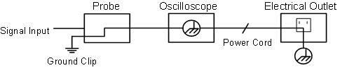
It is not allowed to measure AC power when the AC powered oscilloscope is connected to the AC-powered PC through the ports.

Warning:

To avoid fire or electrical shock, when the oscilloscope input signal connected is more than 42V peak (30Vrms) or on circuits of more than 4800VA, please take note of below items:

• Only use accessory insulated voltage probes and test lead.
  
• Check the accessories such as probe before use and replace it if there are any damages.
  
• Remove probes, test leads and other accessories immediately after use.
  
• Remove USB cable which connects oscilloscope and computer.
  
• Do not apply input voltages above the rating of the instrument because the probe tip voltage will directly transmit to the oscilloscope. Use with caution when the probe is set as 1:1.
  
• Do not use exposed metal BNC or banana plug connectors.
  
• Do not insert metal objects into connectors.
  

3. Quick Start

Introduction to the Structure of the Oscilloscope

This chapter makes a simple description of the operation and function of the front panel of the oscilloscope, enabling you to be familiar with the use of the oscilloscope in the shortest time.

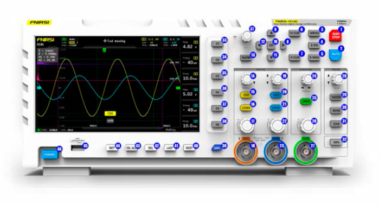
Front Panel

The front panel has knobs and function buttons. The 5 buttons in the column on the right side of the display screen are menu selection buttons, through which, you can set the different options for the current menu. The other buttons are function buttons, through which, you can enter different function menus or obtain a specific function application directly.

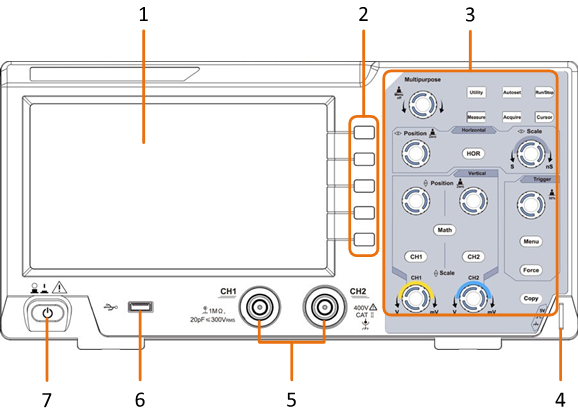
Figure 3-1 Front panel

1. Display area
   
2. Menu selection buttons: Select the right menu item.
   
3. Control (button and knob) area
   
4. Probe Compensation: Measurement signal (5V/1kHz) output.
   
5. Signal Input Channel
   
6. USB Host port: It is used to transfer data when external USB equipment connects to the oscilloscope regarded as “host device”. For example: Saving the waveform to USB flash disk needs to use this port.
   
7. Power on/off
   

Rear Panel

5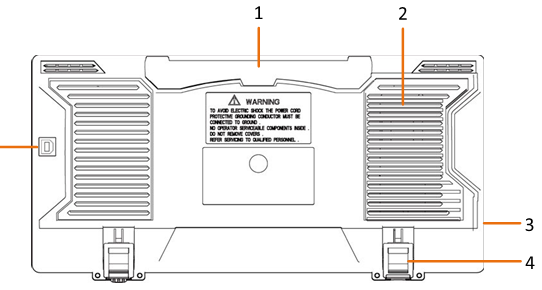

Figure 3-2 Rear Panel

1. Handle
   
2. Air vents
   
3. AC power input jack
   
4. Foot stool: Adjust the tilt angle of the oscilloscope.
   
5. USB Device port: It is used to transfer data when external USB equipment connects to the oscilloscope regarded as “slave device”. For example: to use this port when connect PC to the oscilloscope by USB.
   

Control Area

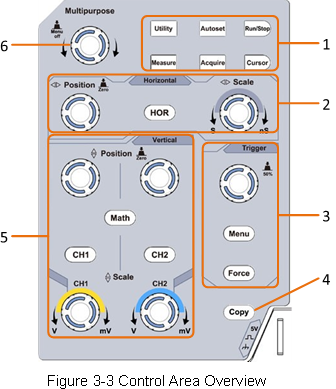
1. Function button area: Total 6 buttons.
   
2. Horizontal control area with 1 button and 2 knobs.
   

   “HOR” button refer to horizontal system setting menu, “Horizontal Position” knob control trigger position, ” Horizontal Scale” control time base.
   

3. Trigger control area with 2 buttons and 1 knob.
   

   The Trigger Level knob is to adjust trigger voltage. Other 2 buttons refer to trigger system setting.
   

4. Copy button: This button is the shortcut for Save function in the Utility function menu. Pressing this button is equal to the Save option in the Save menu. The waveform, configure or the display screen could be saved according to the chosen type in the Save menu.
   
5. Vertical control area with 3 buttons and 4 knobs.
   

   “CH1” and “CH2 ” correspond to setting menu in CH1 and CH2, “Math” button refer to math menu, the math menu consists of six kinds of operations, including CH1-CH2, CH2-CH1, CH1+CH2, CH1*CH2, CH1/CH2 and FFT. Two “Vertical Position” knob control the vertical position of CH1/CH2, and two “Scale” knob control voltage scale of CH1, CH2.
   

6. M knob(Multipurpose knob): when a symbol appears in the menu, it indicates you can turn the M knob to select the menu or set the value. You can push it to close the menu on the left and right.
   

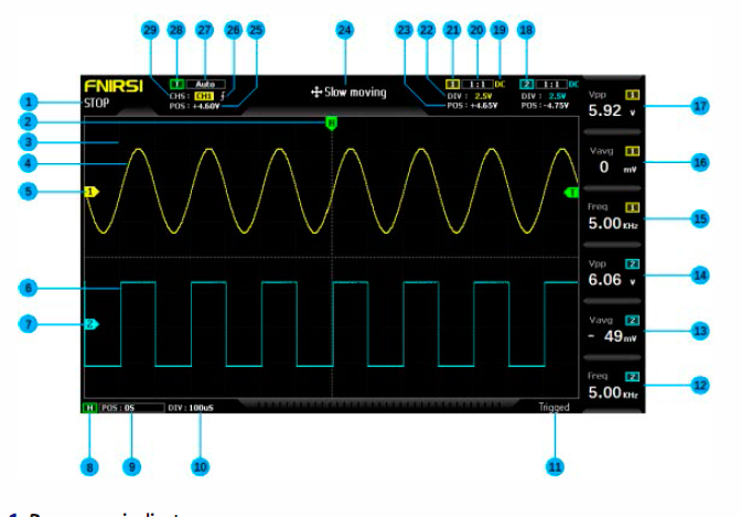
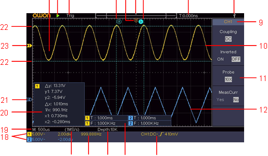
User Interface Introduction

    1 2 3    4 5 64    7    8

    17 16 15 14    13    

Figure 3-4 Illustrative Drawing of Display Interfaces

1. Waveform Display Area. 2. Run/Stop

1. The state of trigger, including:
   

   Auto: Automatic mode and acquire waveform without triggering.
   

   Trig: Trigger detected and acquire waveform.
   

   Ready: Pre-triggered data captured and ready for a trigger.
   

   Scan: Capture and display the waveform continuously.
   

   Stop: Data acquisition stopped.
   

2. The two blue dotted lines indicates the vertical position of cursor measurement.
   
3. The T pointer indicates the horizontal position for the trigger.
   
4. The pointer indicates the trigger position in the record length.
   
5. It shows present triggering value and displays the site of present window in internal memory.
   
6. It indicates that there is a USB disk connecting with the oscilloscope.
   
7. Channel identifier of current menu.
   
8. The waveform of CH1.
   
9. Right Menu.
   
10. The waveform of CH2.
    
11. Current trigger type:
    

         Rising edge triggering

Falling edge triggering

Video line synchronous triggering

         Video field synchronous triggering

The reading shows the trigger level value of the corresponding channel.

1. It indicates the measured type and value of the corresponding channel. “T” means period, “F” means frequency, “V” means the average value, “Vp” the peak-peak value, “Vr” the root-mean-square value, “Ma” the maximum amplitude value, “Mi” the minimum amplitude value, “Vt” the Voltage value of the waveform’s flat top value, “Vb” the Voltage value of the waveform’s flat base, “Va” the amplitude value, “Os” the overshoot value, “Ps” the Preshoot value, “RT” the rise time value, “FT” the fall time value, “PW” the +width value, “NW” the -Width value, “+D” the +Duty value, “-D” the -Duty value, “PD” the Delay A->B value, “ND” the Delay A->B value, “TR” the Cycle RMS, “CR” the Cursor RMS, “WP” the Screen Duty, “RP” the Phase, “+PC” the +Pulse count, “-PC” the – Pulse count, “+E” the Rise edge count, “-E” the Fall edge count, “AR” the Area, “CA” the Cycle area.
   
2. The readings show the record length.
   
3. The frequency of the trigger signal.
   
4. The readings show current sample rate.
   
5. The readings indicate the corresponding Voltage Division and the Zero Point positions of the channels. “BW” indicates bandwidth limit.
   

   The icon shows the coupling mode of the channel.
   

   “—” indicates direct current coupling
   

   “～” indicates AC coupling
   

   “” indicates GND coupling
   

6. The reading shows the setting of main time base.
   
7. It is cursor measure window, showing the absolute values and the readings of the cursors.
   
8. The blue pointer shows the grounding datum point (zero point position) of the waveform of the CH2 channel. If the pointer is not displayed, it means that this channel is not opened.
   
9. The two blue dotted lines indicate the horizontal position of cursor measurement.
   
10. The yellow pointer indicates the grounding datum point (zero point position) of the waveform of the CH1 channel. If the pointer is not displayed, it means that the channel is not opened.
    

How to Implement the General Inspection

After you get a new oscilloscope, it is recommended that you should make a check on the instrument according to the following steps:

1. Check whether there is any damage caused by transportation.
   

   If it is found that the packaging carton or the foamed plastic protection cushion has suffered serious damage, do not throw it away first till the complete device and its accessories succeed in the electrical and mechanical property tests.
   

2. Check the Accessories
   

   The supplied accessories have been already described in the “Appendix A: Enclosure” of this Manual. You can check whether there is any loss of accessories with reference to this description. If it is found that there is any accessory lost or damaged, please get in touch with the distributor of OWON responsible for this service or the OWON’s local offices.
   

3. Check the Complete Instrument
   

   If it is found that there is damage to the appearance of the instrument, or the instrument can not work normally, or fails in the performance test, please get in touch with the OWON’s distributor responsible for this business or the OWON’s local offices. If there is damage to the instrument caused by the transportation, please keep the package. With the transportation department or the OWON’s distributor responsible for this business informed about it, a repairing or replacement of the instrument will be arranged by the OWON.
   

How to Implement the Function Inspection

Make a fast function check to verify the normal operation of the instrument, according to the following steps:

1. Connect the power cord to a power source. Press the
   button on the bottom left of the instrument.
   

The instrument carries out all self-check items and shows the Boot Logo. Push the Utility button, select Function in the right menu. Select Adjust in the left menu, select Default in the right menu. The default attenuation coefficient set value of the probe in the menu is 10X.

1. Set the Switch in the Oscilloscope Probe as 10X and Connect the Oscilloscope with CH1 Channel.
   

Align the slot in the probe with the plug in the CH1 connector BNC, and then tighten the probe with rotating it to the right side.

Connect the probe tip and the ground clamp to the connector of the probe compensator.

1. Push the Autoset Button on the front panel.
   

The square wave of 1 KHz frequency and 5V peak-peak value will be displayed in several seconds (see Figure 3-5).

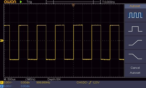
Figure 3-5 Auto set

Check CH2 by repeating Step 2 and Step 3.

How to Implement the Probe Compensation

When connect the probe with any input channel for the first time, make this adjustment to match the probe with the input channel. The probe which is not compensated or presents a compensation deviation will result in the measuring error or mistake. For adjusting the probe compensation, please carry out the following steps:

1. Set the attenuation coefficient of the probe in the menu as 10X and that of the switch in the probe as 10X
   (see “How to Set the Probe Attenuation Coefficient” on P11), and connect the probe with the CH1 channel. If a probe hook tip is used, ensure that it keeps in close touch with the probe. Connect the probe tip with the signal connector of the probe compensator and connect the reference wire clamp with the ground wire connector of the probe connector, and then push the Autoset button on the front panel.
   
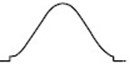
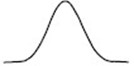
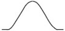
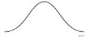
2. Check the displayed waveforms and regulate the probe till a correct compensation is achieved (see Figure 3-6 and Figure 3-7).
   

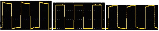
    Overcompensated     Compensated correctly     Under compensated

Figure 3-6 Displayed Waveforms of the Probe Compensation

1. Repeat the steps mentioned if needed.
   

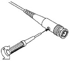
Figure 3-7 Adjust Probe

How to Set the Probe Attenuation Coefficient

The probe has several attenuation coefficients, which will influence the vertical scale factor of the oscilloscope.

To change or check the probe attenuation coefficient in the menu of oscilloscope:

1. Push the function menu button of the used channels (CH1 or CH2 button).
   
2. Select Probe in the right menu; turn the M knob to select the proper value in the left menu corresponding to the probe.
   

This setting will be valid all the time before it is changed again.

The default attenuation coefficient of the probe on the instrument is preset to 10X.

Make sure that the set value of the attenuation switch in the probe is the same as the menu selection of the probe attenuation coefficient in the oscilloscope.

The set values of the probe switch are 1X and 10X (see Figure 3-8).

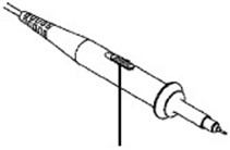
Figure 3-8 Attenuation Switch

When
the attenuation switch is set to 1X, the probe will limit the bandwidth of the oscilloscope in 5MHz. To use the full bandwidth of the oscilloscope, the switch must be set to 10X.

How to Use the Probe Safely

The safety guard ring around the probe body protects your finger against any electric shock, shown as Figure 3-9.

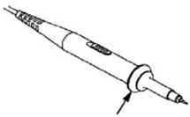
Figure 3-9 Finger Guard

To avoid electric shock, always keep your finger behind the safety guard ring of the probe during the operation.

To protect you from suffering from the electric shock, do not touch any metal part of the probe tip when it is connected to the power supply.

Before making any measurements, always connect the probe to the instrument and connect the ground terminal to the earth.

How to Implement Self-calibration

The self-calibration application can make the oscilloscope reach the optimum condition rapidly to obtain the most accurate measurement value. You can carry out this application program at any time. This program must be executed whenever the change of ambient temperature is 5℃ or over.

Before performing a self-calibration, disconnect all probes or wires from the input connector. Push the Utility button, select Function in the right menu, select Adjust. in the left menu, select Self Cal in the right menu; run the program after everything is ready.

Introduction to the Vertical System

As shown in Figure 3-10, there are a few of buttons and knobs in Vertical Controls. The following practices will gradually direct you to be familiar with the using of the vertical setting.

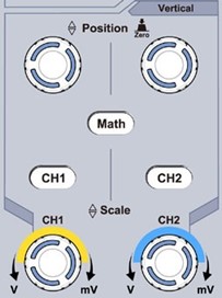
Figure 3-10 Vertical Control Zone

1. Use the Vertical Position knob to show the signal in the center of the waveform window. The Vertical Position knob functions the regulating of the vertical display position of the signal. Thus, when the Vertical Position knob is rotated, the pointer of the earth datum point of the channel is directed to move up and down following the waveform.

Measuring Skill

If the channel is under the DC coupling mode, you can rapidly measure the DC component of the signal through the observation of the difference between the wave form and the signal ground.

If the channel is under the AC mode, the DC component would be filtered out. This mode helps you display the AC component of the signal with a higher sensitivity.

Vertical offset back to 0 shortcut key

Turn the Vertical Position knob to change the vertical display position of channel and push the position knob to set the vertical display position back to 0 as a shortcut key, this is especially helpful when the trace position is far out of the screen and want it to get back to the screen center immediately.

2. Change the Vertical Setting and Observe the Consequent State Information Change.

With the information displayed in the status bar at the bottom of the waveform window, you can determine any changes in the channel vertical scale factor.

• Turn the Vertical
  Scale knob and change the “Vertical Scale Factor (Voltage Division)”, it can be found that the scale factor of the channel corresponding to the status bar has been changed accordingly.
  
• Push buttons of CH1, CH2 and Math, the operation menu, symbols, waveforms and scale factor status information of the corresponding channel will be displayed in the screen.
  

Introduction to the Horizontal System

Shown as Figure 3-11, there are a button and two knobs in the Horizontal
Controls. The following practices will gradually direct you to be familiar with the setting of horizontal time base.

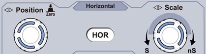
Figure 3-11 Horizontal Control Zone

1. Turn the Horizontal Scale knob to change the horizontal time base setting and observe the consequent status information change. Turn the Horizontal Scale knob to change the horizontal time base, and it can be found that the Horizontal Time Base display in the status bar changes accordingly.
   
2. Use the Horizontal Position knob to adjust the horizontal position of the signal in the waveform window. The Horizontal Position knob is used to control the triggering displacement of the signal or for other special applications. If it is applied to triggering the displacement, it can be observed that the waveform moves horizontally with the knob when you rotate the Horizontal Position knob.
   

   Triggering displacement back to 0 shortcut key
   

   Turn the Horizontal Position knob to change the horizontal position of channel and push the Horizontal Position knob to set the triggering displacement back to 0 as a shortcut key.
   

3. Push the Horizontal HOR button to switch between the normal mode and the wave zoom mode.
   

Introduction to the Trigger System

As shown in Figure 3-12, there are one knob and three buttons make up Trigger
Controls. The following practices will direct you to be familiar with the setting of the trigger system gradually.

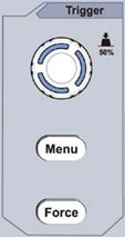
Figure 3-12 Trigger Control Zone

1. Push the Trigger Menu button and call out the trigger menu. With the operations of the menu selection buttons, the trigger setting can be changed.
   
2. Use the Trigger Level knob to change the trigger level setting.
   

   By turning the Trigger Level knob, the trigger indicator in the screen will move up and down. With the movement of the trigger indicator, it can be observed that the trigger level value displayed in the screen changes accordingly.
   

   Note: Turning the Trigger Level knob can change trigger level value and it is also the hotkey to set trigger level as the vertical mid point values of the amplitude of the trigger signal.
   

3. Push the Force button to force a trigger signal, which is mainly applied to the
   

   “Normal” and “Single” trigger modes.
   

4. Advanced User Guidebook

This chapter will deal with the following topics mainly:

• How to Set the Vertical System
  
• How to Set the Horizontal System
  
• How to Set the Trigger System
  
• How to Set the Sampling/Display
  
• How to Save and Recall Waveform
  
• How to Implement the Auxiliary System Function Setting
  
• How to Update your Instrument Firmware
  
• How to Measure Automatically
  
• How to Measure with Cursors
  
• How to Use Executive Buttons
  

It is recommended that you read this chapter carefully to get acquainted the various measurement functions and other operation methods of the oscilloscope.

How to Set the Vertical System

The VERTICAL CONTROLS includes three menu buttons such as CH1, CH2 and Math,
and four knobs such as Vertical Position, Vertical Scale for each channel.

Setting of CH1 and CH2

Each channel has an independent vertical menu and each item is set respectively based on the channel.

To turn waveforms on or off (channel, math)

Pushing the CH1, CH2, or Math buttons have the following effect:

• If the waveform is off, the waveform is turned on and its menu is displayed.
  
• If the waveform is on and its menu is not displayed, its menu will be displayed.
  
• If the waveform is on and its menu is displayed, the waveform is turned off and its menu goes away.
  

The description of the Channel Menu is shown as the following list:

1. To set channel coupling
   

   Taking the Channel 1 for example, the measured signal is a square wave signal containing the direct current bias. The operation steps are shown as below:
   

   1. Push the CH1 button to show the CH1 SETUP menu.
      
   2. In the right menu, select Coupling as DC. Both DC and AC components of the signal are passed.
      
   3. In the right menu, select Coupling as AC. The direct current component of the signal is blocked.
      
2. To invert a waveform
   

   Waveform inverted: the displayed signal is turned 180 degrees against the phase of the earth potential.
   

   Taking the Channel 1 for example, the operation steps are shown as follows:
   

   1. Push the CH1 button to show the CH1 SETUP menu.
      
   2. In the right menu, select Inverted as ON, the waveform is inverted. Push again to switch to OFF, the waveform goes back to its original one.
      
3. To adjust the probe attenuation
   

   For correct measurements, the attenuation coefficient settings in the operating menu of the Channel should always match what is on the probe (see “How to Set the Probe Attenuation Coefficient” on P11). If the attenuation coefficient of the probe is 1:1, the menu setting of the input channel should be set to1X.
   

   Take the Channel 1 as an example, the attenuation coefficient of the probe is 10:1, the operation steps are shown as follows:
   

   1. Push the CH1 button to show the CH1 SETUP menu.
      
   2. In the right menu, select Probe. In the left menu, turn the M knob to set it as 10X.
      
4. To measure current by probing the voltage drop across a resistor
   

   Take the Channel 1 as an example, if you are measuring current by probing the voltage drop across a 1Ω resistor, the operation steps are shown as follows:
   

   1. Push the CH1 button to show CH1 SETUP menu.
      
   2. In the right menu, set MeasCurr as Yes, the A/V radio menu will appear below. Select it; turn the M knob to set the Amps/Volts ratio. Amps/Volts ratio = 1/Resistor value. Here the A/V radio should be set to 1.
      

Use Mathematical Manipulation Function

The Mathematical Manipulation function is
used to show the results of the addition, multiplication, division and subtraction operations between two channels, or the FFT operation for a channel. Press the Math button to display the menu on the right.

The Waveform Calculation

Press the Math button to display the menu on the right, select Type as Math.

Taking the additive operation between Channel 1 and Channels 2 for example, the operation steps are as follows:

1. Press the Math button to display the math menu in the right. The pink M waveform appears on the screen.
   
2. In the right menu, select Type as Math.
   
3. In the right menu, select Factor1 as CH1.
   
4. In the right menu, select Sign as +.
   
5. In the right menu, select Factor2 as CH2.
   
6. Press Next Page in the right menu. Select Vertical (div), thesymbol is in front of div, turn the M knob to adjust the vertical position of Math waveform.
   
7. Select Vertical (V/div) in the right menu, thesymbol is in front of the voltage, turn the M knob to adjust the voltage division of Math waveform.
   

Using FFT function

The FFT (fast Fourier transform) math function mathematically converts a time-domain waveform into its frequency components. It is very useful for analyzing the input signal on Oscilloscope. You can match these frequencies with known system frequencies, such as system clocks, oscillators, or power supplies.

FFT function in this oscilloscope transforms 2048 data points of the time-domain signal into its frequency components mathematically (the record length should be 10K or above). The final frequency contains 1024 points ranging from 0Hz to Nyquist frequency.

Press the Math button to display the menu on the right, select Type as FFT.

Taking the FFT operation for example, the operation steps are as follows:

1. Press the Math button to display the math menu in the right.
   
2. In the right menu, select Type as FFT.
   
3. In the right menu, select Source as CH1.
   
4. In the right menu, select Window. Select the proper window type in the left menu.
   
5. In the right menu, select Format as Vrms or dB.
   
6. In the right menu, press Hori (Hz) to make thesymbol in front of the frequency value, turn the M knob to adjust the horizontal position of FFT waveform; then press to make thesymbol in front of the frequency/div below, turn the M knob to adjust the time base of FFT waveform.
   
7. Select Vertical in the right menu; do the same operations as above to set the vertical position and voltage division.
   

To select the FFT window

■ There are 6 FFT windows. Each one has trade-offs between frequency resolution and magnitude accuracy. What you want to measure and your source signal characteristics help you to determine which window to use. Use the following guidelines to select the best window.

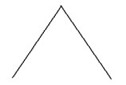Notes for using FFT

• Use the default dB scale for details of multiple frequencies, even if they have very different amplitudes. Use the Vrms scale to compare frequencies.
  
• DC component or offset can cause incorrect magnitude values of FFT waveform. To minimize the DC component, choose AC Coupling on the source signal.
  
• To reduce random noise and aliased components in repetitive or single-shot events, set the oscilloscope acquisition mode to average.
  

What is Nyquist frequency?

The Nyquist frequency is the highest frequency that any real-time digitizing oscilloscope can acquire without aliasing. This frequency is half of the sample rate. Frequencies above the Nyquist frequency will be under sampled, which causes aliasing. So pay more attention to the relation between the frequency being sampled and measured.

Use Vertical Position and Scale Knobs

1. The Vertical Position knob is used to adjust the vertical positions of the waveforms.
   

   The analytic resolution of this control knob changes with the vertical division.
   

2. The Vertical Scale knob is used to regulate the vertical resolution of the wave forms. The sensitivity of the vertical division steps as 1-2-5.
   

The vertical position and vertical resolution is displayed at the left bottom corner of the screen (see Figure 4-1).

Figure 4-1 Information about Vertical Position

How to Set the Horizontal System

The HORIZONTAL CONTROLS includes the Horizontal HOR button and such knobs as Horizontal Position and Horizontal Scale.

1. Horizontal Position knob: this knob is used to adjust the horizontal positions of all channels (include those obtained from the mathematical manipulation), the analytic resolution of which changes with the time base.
   
2. Horizontal Scale knob: it is used to set the horizontal scale factor for setting the main time base or the window.
   
3. Horizontal HOR button: push it to switch between the normal mode and the wave zoom mode. For more detailed operations, see the introductions below.
   

Zoom the Waveform

Push the Horizontal
HOR button to enter wave zoom mode. The top half of the display shows the Main window and the bottom half displays the Zoom window. The Zoom window is a magnified portion of the Main window.

Selected portion

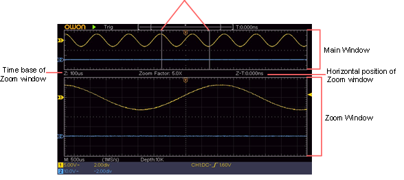
In normal mode, the Horizontal Position and Horizontal Scale knobs are used to adjust the horizontal position and time base of the Main window.

In wave zoom mode, the Horizontal Position and Horizontal Scale knobs are used to adjust the horizontal position and time base of the Zoom window.

How to Set the Trigger System

Trigger determines when DSO starts to acquire data and display waveform. Once trigger is set correctly, it can convert the unstable display to meaningful waveform. When DSO starts to acquire data, it will collect enough data to draw waveform on left of trigger point. DSO continues to acquire data while waiting for trigger condition to occur. Once it detects a trigger it will acquire enough data continuously to draw the waveform on right of trigger point.

Trigger control area consists of 1 knob and 2 menu buttons.

Trigger Level: The knob that set the trigger level; push the knob and the level will be set as the vertical mid point values of the amplitude of the trigger signal.

Force: Force to create a trigger signal and the function is mainly used in “Normal” and “Single” mode.

Trigger Menu: The button that activates the trigger control menu.

Trigger Control

The oscilloscope provides two trigger types: single trigger, alternate trigger. Each type of trigger has different sub menus.

Single trigger: Use a trigger level to capture stable waveforms in two channels simultaneously.

Alternate trigger: Trigger on non-synchronized signals.

The Single Trigger, Alternate Trigger menus are described respectively as follows:

Single Trigger

Single trigger has two types: edge trigger, video trigger.

Edge Trigger: It occurs when the trigger input passes through a specified voltage level with the specified slope.

Video Trigger: Trigger on fields or lines for standard video signal.

The two trigger modes in Single Trigger are described respectively as follows:

1. Edge Trigger

An edge trigger occurs on trigger level value of the specified edge of input signal. Select Edge trigger mode to trigger on rising edge or falling edge.

Push the Trigger Menu button to display the Trigger
menu on the right. Select Type as Single in the right menu. Select Single as Edge in the right menu.

In Edge Trigger mode, the trigger setting information is displayed on bottom right of the

screen, for example,     indicates that trigger type is edge, trigger

source is CH1, coupling is DC, and trigger level is 0.00mV.

Edge menu list:

Trigger Level: trigger level indicates vertical trig position of the channel, rotate trig level knob to move trigger level, during setting, a dotted line displays to show trig position, and the value of trigger level changes at the right corner, after setting, dotted line disappears.

2. Video Trigger

Choose video trigger to trigger on fields or lines of NTSC, PAL or SECAM standard video signals.

Push the Trigger Menu button to display the Trigger
menu on the right. Select Type as Single in the right menu. Select Single as Video in the right menu.

In Video Trigger mode, the trigger setting information is displayed on bottom right of the screen, for example, indicates that trigger type is Video, trigger source is

CH1, and Sync type is Even.

Video Trigger menu list:

Alternate Trigger (Trigger mode: Edge)

Trigger signal comes from two vertical channels when alternate trigger is on. This mode is used to observe two unrelated signals. Trigger mode is edge trigger.

Alternate trigger (Trigger Type: Edge)
menu list:

How to Operate the Function Menu

The function menu control zone includes 4 function menu buttons: Utility, Measure, Acquire, Cursor, and 2 immediate-execution buttons: Autoset, Run/Stop.

How to Set the Sampling/Display

Push the Acquire button, the Sampling and Display menu is shown in the right as follows:

Average

Normal sampling mode.

Use to capture maximal and minimal samples. Finding highest and lowest points over adjacent intervals. It is used for the detection of the jamming burr and the possibility of reducing the confusion.

It is used to reduce the random and don’t-care noises, with the optional number of averages. Turn the M knob to select 4, 16, 64, 128 in the left menu.

Type

Dots

Vect

Only the sampling points are displayed.

The space between the adjacent sampling points in the display is filled with the vector form.

Persist

OFF

1. Second
   
2. Seconds
   

5 Seconds

Infinity

Set the persistence time

XY Mode

ON

OFF

Turn on/off XY display function

Counter

ON

OFF

Turn on/off counter

 

Persist

When the Persist function is used, the persistence display effect of the picture tube oscilloscope can be simulated. The reserved original data is displayed in fade color and the new data is in bright color.

1. Push the Acquire button.
   
2. In the right menu, press Persist to select the persist time, including OFF, 1 Second, 2 Seconds, 5 Seconds and Infinity.
   When the “Infinity” option is set for Persist
   Time, the measuring points will be stored till the controlling value is changed. Select OFF to turn off persistence and clear the display.
   

XY Format

This format is only applicable to Channel 1 and Channel 2. After the XY display format is selected, Channel 1 is displayed in the horizontal axis and Channel 2 in the vertical axis; the oscilloscope is set in the un-triggered sample mode: the data are displayed as bright spots.

The operations of all control knobs are as follows:

• The Vertical Scale and the Vertical Position knobs of Channel 1 are used to set the horizontal scale and position.
  
• The Vertical Scale and the Vertical Position knobs
  of Channel 2 are used to set the vertical scale and position continuously.
  

The following functions can not work in the XY Format:

• Reference or digital wave form
  
• Cursor
  
• Trigger control
  
• FFT
  

Operation steps:

1. Push the Acquire button to show the right menu.
   
2. Select XY Mode as ON or OFF in the right menu.
   

Counter

It is a 6-digit single-channel counter. The counter can only measure the frequency of the triggering channel. The frequency range is from 2Hz to the full bandwidth. Only if the measured channel is in Edge mode of Single trigger type, the counter can be enabled. The counter is displayed at the bottom of the screen.

Operation steps:

1. Push Trigger Menu button, set the trigger type to Single, set the trigger mode to Edge, select the signal source.
   
2. Push the Acquire button to show the right menu.
   
3. Select Counter as ON or OFF in the right menu.
   

How to Save and Recall a Waveform

Push the Utility button, select Function in the right menu, select Save in the left menu.

By selecting Type in the right menu, you can save the waveforms, configures or screen images.

When the Type is selected as Wave, the menu is shown as the following table:

When the Type is selected as Configure, the menu is shown as the following table:

When the Type is selected as Image, the menu is shown as the following table:

Save and Recall the Waveform

The oscilloscope can store 16 waveforms, which can be displayed with the current waveform at the same time. The stored waveform called out can not be adjusted.

In order to save the waveform of CH1, CH2 and Math into the address 1, the operation steps should be followed:

1. Turn on CH1, CH2 and Math channels.
   
2. Push the Utility button, select Function in the right menu, select Save in the left menu. In the right menu, select Type as Wave.
   
3. Saving: In the right menu, select Source as All.
   
4. In the right menu, press Object. Select 1 as object address in the left menu.
   
5. In the right menu, press Next Page, and select Storage as Internal.
   
6. In the right menu, press Save to save the waveform.
   
7. Recalling: In the right menu, press Prev Page, and press Object, select 1 in the left menu. In the right menu, select Object as ON, the waveform stored in the address will be shown, the address number and relevant information will be displayed at the top left of the screen.
   

In order to save the waveform of CH1 and CH2 into the USB storage as a BIN file, the operation steps should be followed:

1. Turn on CH1 and CH2 channels, turn off the Math channel.
   
2. Push the Utility button, select Function in the right menu, select Save in the left menu. In the right menu, select Type as Wave.
   
3. Saving: In the right menu, select Source as All.
   
4. In the right menu, press Next Page, and select File Format as BIN.
   
5. In the right menu, select Storage as External.
   
6. In the right menu, select Storage, an input keyboard used to edit the file name will pop up. The default name is current system date and time. Turn the M knob to choose the keys; press the M knob to input the chosen key. The length of file name is up to 25 characters. Select the key in the keyboard to confirm.
   
7. Recalling: The BIN waveform file could be open by OWON waveform analysis software (on the supplied CD).
   

Shortcut for Save
function:

The Copy button on the bottom right of the front panel is the shortcut for Save function in the Utility function menu. Pressing this button is equal to the Save option in the Save menu. The waveform, configure or the display screen could be saved according to the chosen type in the Save menu.

Save the current screen image:

The screen image can only be stored in USB disk, so you should connect a USB disk with the instrument.

1. Install the USB disk: Insert the USB disk into the “7. USB Host port” of “Figure 3-1 Front panel“. If an icon appears on the top right of the screen, the USB disk is installed successfully. If the USB disk cannot be recognized, format the USB disk according to the methods in “USB disk Requirements” on P31.
   
2. After the USB disk is installed, push the Utility button, select Function in the right menu, select Save in the left menu. In the right menu, select Type as Image.
   
3. Select Save in the right menu, an input keyboard used to edit the file name will pop up. The default name is current system date and time. Turn the M knob to choose the keys; press the M knob to input the chosen key. The length of file name is up to 25 characters. Select the key in the keyboard to confirm.
   

USB disk Requirements

The supported format of the USB disk: FAT32 file system, the allocation unit size cannot exceed 4K, mass storage USB disk is also supported. If the USB disk doesn’t work properly, format it into the supported format and try again. Follow any of the following two methods to format the USB disk: using system-provided function and using the formatting tools. (The USB disk of 8 G or 8 G above can only be formatted using the second method – using the formatting tools.)

Use system-provided function to format the USB disk

1. Connect the USB disk to the computer.
   
2. Right click Computer- Manage to enter Computer Management interface.
   
3. Click Disk Management menu, and information about the USB disk will display on the right side with red mark 1 and 2.
   

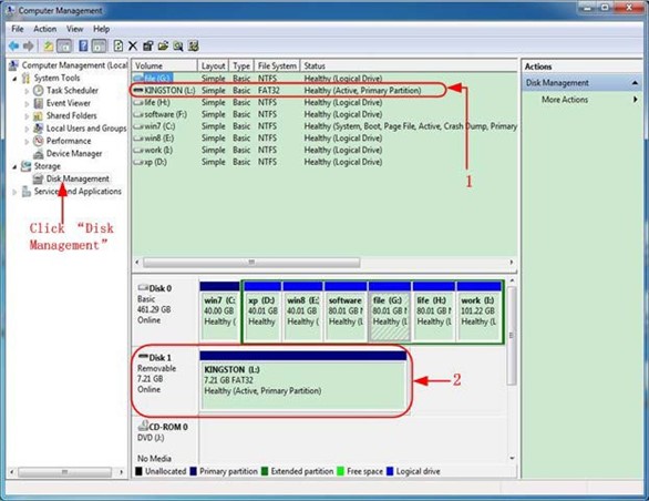
Figure 4-2: Disk Management of computer

1. Right click 1 or 2 red mark area, choose Format. And system will pop up a warning message, click Yes.
   

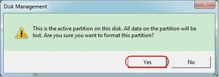
Figure 4-3: Format the USB disk warning

1. Set File System as FAT32, Allocation unit size 4096. Check “Perform a quick
   format” to execute a quick format. Click OK, and then click Yes on the warning message.
   

   
   

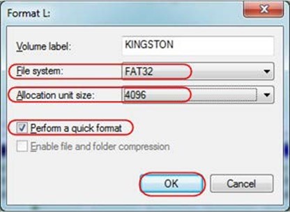
Figure 4-4: Formatting the USB disk setting 6. Formatting process.

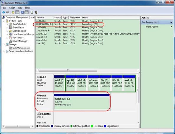
Figure 4-5: Formatting the USB disk

7.     Check whether the USB disk is FAT32 with allocation unit size 4096 after formatting.

Use Minitool Partition Wizard to format

Download URL:
http://www.partitionwizard.com/free-partition-manager.html

Tip: There are many tools for the USB disk formatting on the market, just take Minitool Partition Wizard for example here.

1. Connect the USB disk to the computer.
   
2. Open the software Minitool Partition Wizard.
   
3. Click Reload Disk on the pull-down menu at the top left or push keyboard F5, and information about the USB disk will display on the right side with red mark 1 and 2.
   

   
   

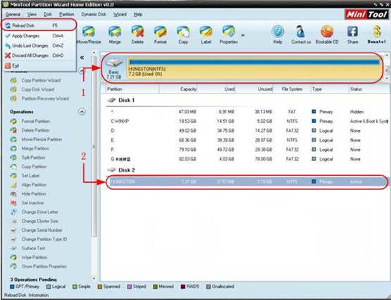
Figure 4-6: Reload Disk 4. Right click 1 or 2 red mark area, choose Format.

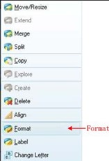
Figure 4-7: Choose format 5. Set File System FAT32, Cluster size 4096. Click OK.

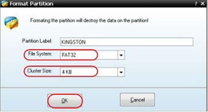
Figure 4-8: Format setting

1. Click Apply at the top left of the menu. Then click Yes on the pop-up warning to begin formatting.
   

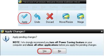
Figure 4-9: Apply setting

1. Formatting process
   

   
   

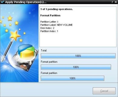
Figure 4-10: Format process

1. Format the USB disk successfully
   

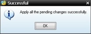
Figure 4-11: Format successfully

How to Implement the Auxiliary System Function Setting

●Config

Push the Utility button, select Function in the right menu, select Configure in the left menu.

The description of Configure Menu is shown as the follows:

●Display

Push the Utility button, select Function in the right menu, select Display in the left menu.

The description of Display
Menu is shown as the follows:

●Adjust

Push the Utility button, select Function in the right menu, select Adjust in the left menu.

The description of Adjust
Menu is shown as the follows:

Do Self Cal (Self-Calibration)

The self-calibration procedure can improve the accuracy of the oscilloscope under the ambient temperature to the greatest extent. If the change of the ambient temperature is up to or exceeds 5℃, the self-calibration procedure should be executed to obtain the highest level of accuracy.

Before executing the self-calibration procedure, disconnect all probes or wires from the input connector. Push the Utility button, select Function in the right menu, the function menu will display at the left, select Adjust. If everything is ready, select Self Cal in the right menu to enter the self-calibration procedure of the instrument.

Probe checking

To check whether probe attenuation is good. The results contain three circumstances: Overflow compensation, Good compensation, Inadequate compensation. According to the checking result, users can adjust probe attenuation to the best. Operation steps are as follows:

1. Connect the probe to CH1, adjust the probe attenuation to the maximum.
   
2. Push the Utility button, select Function in the right menu, select Adjust in the left menu.
   
3. Select ProbeCh. in the right menu, tips about probe checking shows on the screen.
   
4. Select ProbeCh. again to begin probe checking and the checking result will occur after 3s; push any other key to quit.
   

● Save

You can save the waveforms, configures or screen images. Refer to “How to Save and Recall a Waveform” on page 28.

● Update

Use the front-panel USB port to update your instrument firmware using a USB memory device. Refer to “How to Update your Instrument Firmware” on page 37.

How to Update your Instrument Firmware

Use the front-panel USB port to update your instrument firmware using a USB memory device.

USB memory device requirements: Insert a USB memory device into the USB port on the front panel. If the icon appears on the top right of the screen, the USB memory

device is installed successfully. If the USB memory device cannot be detected, format the USB memory device according to the methods in “USB disk Requirements” on P31.

Caution: Updating your instrument firmware is a sensitive operation, to prevent damage to the instrument, do not power off the instrument or remove the USB memory device during the update process.

To update your instrument firmware, do the following:

1. Push the Utility button, select Function in the right menu, select Configure in the left menu, select About in the right menu. View the model and the currently installed firmware version.
   
2. From a PC, visit www.owon.com.cn and check if the website offers a newer firmware version. Download the firmware file. The file name must be Scope.update. Copy the firmware file onto the root directory of your USB memory device.
   
3. Insert the USB memory device into the front-panel USB port on your instrument.
   
4. Push the Utility button, select Function in the right menu, select Update in the left menu.
   
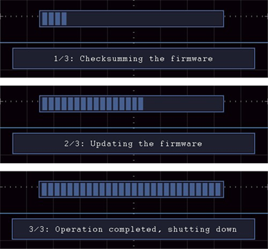
5. In the right menu, select Start, the messages below will be shown.
   

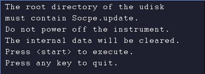
1. In the right menu, select Start again, the interfaces below will be displayed in sequence. The update process will take up to three minutes. After completion, the instrument will be shut down automatically.
   

   
   

2. Press the
   button to power on the instrument.
   

How to Measure Automatically

Push the Measure button to display the menu for the settings of the Automatic Measurements. At most 8 types of measurements could be displayed on the bottom left of the screen.

The oscilloscopes provide 30 parameters for auto measurement, including Period,

Frequency, Mean, PK-PK, RMS, Max, Min, Top, Base, Amplitude, Overshoot, Preshoot,

Rise Time, Fall Time, +PulseWidth, -PulseWidth, +Duty Cycle, -Duty Cycle, Delay A→B, Delay A→B, Cycle RMS, Cursor RMS, Screen Duty, Phase, +PulseCount, -PulseCount, RiseEdgeCnt, FallEdgeCnt, Area, and Cycle Area.

The “Automatic Measurements” menu is described as the following table:

Measure

Only if the waveform channel is in the ON state, the measurement can be performed. The automatic measurement can not be performed in the following situation: 1) On the saved waveform. 2) On the Dual Wfm Math waveform. 3) On the Video trigger mode.

On the Scan format, period and frequency can not be measured.

Measure the period, the frequency of the CH1, following the steps below:

1. Push the Measure button to show the right menu.
   
2. Select AddCH1 in the right menu.
   
3. In the left Type menu, turn the M knob to select Period.
   
4. In the right menu, select AddCH1. The period type is added.
   
5. In the left Type menu, turn the M knob to select Frequency.
   
6. In the right menu, select AddCH1. The frequency type is added.
   

The measured value will be displayed at the bottom left of the screen automatically (see Figure 4-12).

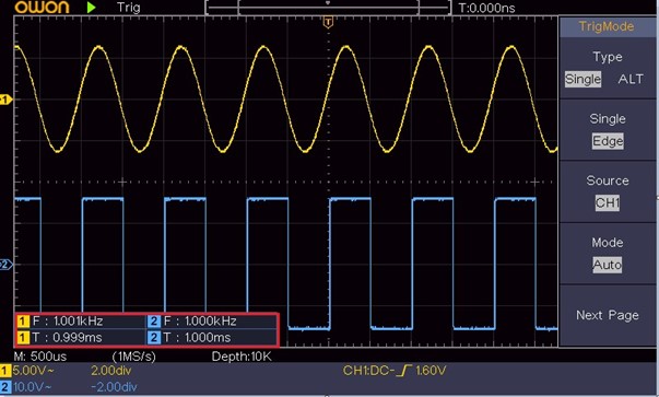
Figure 4-12 Automatic measurement

The automatic measurement of voltage parameters

The oscilloscopes provide automatic voltage measurements including Mean, PK-PK, RMS, Max, Min, Vtop, Vbase, Vamp, OverShoot, PreShoot, Cycle RMS, and Cursor

RMS. Figure 4-13 below shows a pulse with some of the voltage measurement points.

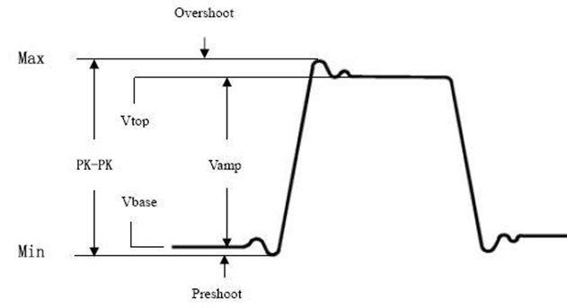
Figure 4-13

Mean: The arithmetic mean over the entire waveform.

PK-PK: Peak-to-Peak Voltage.

RMS: The true Root Mean Square voltage over the entire waveform.

Max: The maximum amplitude. The most positive peak voltage measured over the entire waveform.

Min: The minimum amplitude. The most negative peak voltage measured over the entire waveform.

Vtop: Voltage of the waveform’s flat top, useful for square/pulse waveforms.

Vbase: Voltage of the waveform’s flat base, useful for square/pulse waveforms.

Vamp: Voltage between Vtop and Vbase of a waveform.

OverShoot: Defined as (Vmax-Vtop)/Vamp, useful for square and pulse waveforms.

PreShoot: Defined as (Vmin-Vbase)/Vamp, useful for square and pulse waveforms.

Cycle RMS: The true Root Mean Square voltage over the first entire period of the waveform.

Cursor RMS: The true Root Mean Square voltage over the range of two cursors.

The automatic measurement of time parameters

The oscilloscopes provide time parameters auto-measurements include Period, Frequency, Rise Time, Fall Time, +D width, -D width, +Duty, -Duty, Delay A→B, Delay A→B, and Duty cycle.

Figure 4-14 shows a pulse with some of the time measurement points.

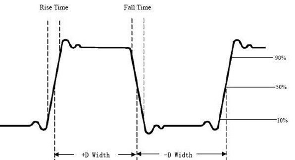
Figure 4-14

Rise Time: Time that the leading edge of the first pulse in the waveform takes to rise from 10% to 90% of its amplitude.

Fall Time: Time that the falling edge of the first pulse in the waveform takes to fall from 90% to 10% of its amplitude.

+D width: The width of the first positive pulse in 50% amplitude points.

-D width: The width of the first negative pulse in the 50% amplitude points.

+Duty: +Duty Cycle, defined as +Width/Period.

-Duty:-Duty Cycle, defined as -Width/Period.

Delay A→B: The delay between the two channels at the rising edge.

Delay A→B: The delay between the two channels at the falling edge.

Screen Duty: Defines as (the width of the positive pulse)/(Entire period)

Phase: Compare the rising edge of CH1 and CH2, calculate phase difference of two channels.

Phase difference=(Delay between channels at the rising edge÷Period)×360°.

Other measurements

+PulseCount : The number of positive pulses that rise above the mid reference crossing in the waveform.

-PulseCount : The number of negative pulses that fall below the mid reference crossing in the waveform.

RiseEdgeCnt : The number of positive transitions from the low reference value to the high reference value in the waveform.

FallEdgeCnt : The number of negative transitions from the high reference value to the low reference value in the waveform.

Area: The area of the whole waveform within the screen and the unit is voltage-second. The area measured above the zero reference (namely the vertical offset) is positive; the area measured below the zero reference is negative. The area measured is the algebraic sum of the area of the whole waveform within the screen.

Cycle Area: The area of the first period of waveform on the screen and the unit is voltage-second. The area above the zero reference (namely the vertical offset) is positive and the area below the zero reference is negative. The area measured is the algebraic sum of the area of the whole period waveform.

Note: When the waveform on the screen is less than a period, the period area measured is 0.

How to Measure with Cursors

Push the Cursor button to turn cursors on and display the cursor menu. Push it again to turn cursors off.

The Cursor Measurement for normal mode:

The description of the cursor menu is shown as the following table:

Perform the following operation steps for the time and voltage cursor measurement of the channel CH1:

1. Push Cursor to display the cursor menu.
   
2. In the right menu, select Source as CH1.
   
3. Press the first menu item in the right menu, select Time&Voltage for Type, two blue dotted lines displayed along the horizontal direction of the screen, two blue dotted lines displayed along the vertical direction of the screen. Cursor measure window at the left bottom of the screen shows the cursor readout.
   
4. In the right menu, select Line Type as Time to make the vertical cursors active. If the Line in the right menu is select as a, turn the M knob to move line a to the right or left. If b is selected, turn the M knob to move line b.
   
5. In the right menu, select Line Type as Voltage to make the horizontal cursors active. Select Line in the right menu as a or b, turn the M knob to move it.
   
6. Push the
   horizontal HOR button to enter wave zoom mode. Push Cursor to show the right menu, select Window as Main or Extension to make the cursors shown in the main window or zoom window.
   

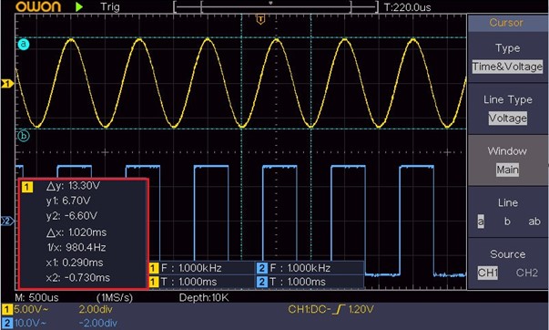
Figure 4-15 Time&Voltage Cursor Measurement

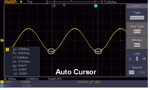
Auto Cursor

For the AutoCursr type, the horizontal cursors are set as the intersections of the vertical cursors and the waveform.

The Cursor Measurement for FFT mode

In FFT mode, push the Cursor button to turn cursors on and display the cursor menu.

The description of the cursor menu in FFT mode is shown as the following table:

Perform the following operation steps for the amplitude and frequency cursor measurement of math FFT:

1. Press the Math button to display the right menu. Select Type as FFT.
   
2. Push Cursor to display the cursor menu.
   
3. In the right menu, select Window as Extension.
   
4. Press the first menu item in the right menu, select Freq&Vamp for Type, two blue dotted lines displayed along the horizontal direction of the screen, two blue dotted lines displayed along the vertical direction of the screen. Cursor measure window at the left bottom of the screen shows the cursor readout.
   
5. In the right menu, select Line Type as Freq to make the vertical cursors active. If the Line in the right menu is select as a, turn the M knob to move line a to the right or left. If b is selected, turn the M knob to move line b.
   
6. In the right menu, select Line Type as Vamp to make the horizontal cursors active. Select Line in the right menu as a or b, turn the M knob to move it.
   
7. In the right cursor menu, you can select Window as Main to make the cursors shown in the main window.
   

How to Use Executive Buttons

Executive Buttons include Autoset, Run/Stop, Copy.

 [Autoset] button

It’s a very useful and quick way to apply a set of pre-set functions to the incoming signal, and display the best possible viewing waveform of the signal and also works out some measurements for user as well.

The details of functions applied to the signal when using Autoset are shown as the following table:

Judge waveform type by Autoset

Five kinds of types: Sine, Square, video signal, DC level, Unknown signal.

Menu as follow:

Description for some icons:

    Multi-period     To display multiple periods

    Single-period         To display single period

    FFT         Switch to FFT mode

    Rising Edge         Display the rising edge of square waveform

    Falling Edge         Display the falling edge of square waveform

    Cancel Autoset    Go back to display the upper menu and waveform information

Note: The Autoset
function requires that the frequency of signal should be no lower

than 20Hz, and the amplitude should be no less than 5mv. Otherwise, the Autoset function may be invalid.

 [Run/Stop] button

Enable or disable sampling on input signals.

Notice: When there is no sampling at STOP state, the vertical division and the horizontal time base of the waveform still can be adjusted within a certain range, in other words, the signal can be expanded in the horizontal or vertical direction. When the horizontal time base is 50ms, the horizontal time base can be expanded for 4 divisions downwards.

 [Copy] button

This button is the shortcut for Save function in the Utility function menu. Pressing this button is equal to the Save option in the Save menu. The waveform, configure or the display screen could be saved according to the chosen type in the Save menu. For more details, please see “How to Save and Recall a Waveform” on P28.

5.Communication with PC

5. Communication with PC

The oscilloscope supports communications with a PC through USB. You can use the Oscilloscope communication software to store, analyze, display the data and remote control.

To learn about how to operate the software, you can push F1 in the software to open the help document.

Here is how to connect with PC via USB port.

1. Install the software: Install the Oscilloscope communication software on the supplied CD.
   
2. Connection: Use a USB data cable to connect the USB Device port in the right panel of the Oscilloscope to the USB port of a PC.
   
3. Install the driver: Run the Oscilloscope communication software on PC, push F1 to open the help document. Follow the steps of title “I. Device connection” in the document to install the driver.
   
4. Port setting of the software: Run the Oscilloscope software; click “Communications” in the menu bar, choose “Ports-Settings”, in the setting dialog, choose “Connect using” as “USB”. After connect successfully, the connection information in the bottom right corner of the software will turn green.
   

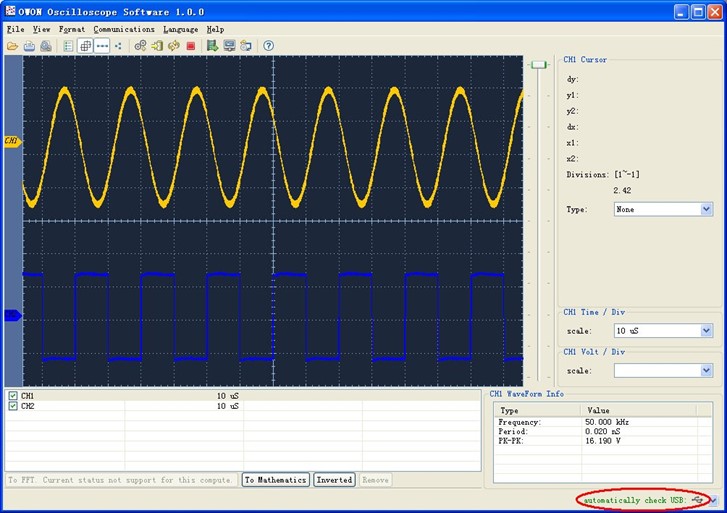
Figure 5-1 Connect with PC through USB port

6. Demonstration

Example 1: Measurement a Simple Signal

The purpose of this example is to display an unknown signal in the circuit, and measure the frequency and peak-to-peak voltage of the signal.

    1.     Carry out the following operation steps for the rapid display of this signal:

1. Set the probe menu attenuation coefficient as 10X and that of the switch in the probe switch as 10X (see “How to Set the Probe Attenuation Coefficient” on P11).
   
2. Connect the probe of Channel 1 to the measured point of the circuit.
   
3. Push the Autoset button.
   

The oscilloscope will implement the Autoset to make the waveform optimized, based on which, you can further regulate the vertical and horizontal divisions till the waveform meets your requirement.

    2.     Perform Automatic Measurement

The oscilloscope can measure most of the displayed signals automatically. To measure the period, the frequency of the CH1, following the steps below:

1. Push the Measure button to show the right menu.
   
2. Select AddCH1 in the right menu.
   
3. In the left Type menu, turn the M knob to select Period.
   
4. In the right menu, select AddCH1. The period type is added.
   
5. In the left Type menu, turn the M knob to select Frequency.
   
6. In the right menu, select AddCH1. The frequency type is added.
   

The measured value will be displayed at the bottom left of the screen automatically (see Figure 6-1).

Figure 6-1 Measure period and frequency value for a given signal

Example 2: Gain of a Amplifier in a Metering Circuit

The purpose of this example is to work out the Gain of an Amplifier in a Metering Circuit. First we use Oscilloscope to measure the amplitude of input signal and output signal from the circuit, then to work out the Gain by using given formulas.

Set the probe menu attenuation coefficient as 10X and that of the switch in the probe as 10X (see “How to Set the Probe Attenuation Coefficient” on P11).

Connect the oscilloscope CH1 channel with the circuit signal input end and the CH2 channel to the output end.

Operation Steps:

1. Push the Autoset button and the oscilloscope will automatically adjust the waveforms of the two channels into the proper display state.
   
2. Push the Measure button to show the right menu.
   
3. Select AddCH1 in the right menu.
   
4. In the left Type menu, turn the M knob to select PK-PK.
   
5. In the right menu, select AddCH1. The peak-to-peak type of CH1 is added.
   
6. In the right menu, select AddCH2. The peak-to-peak type of CH2 is added.
   
7. Read the peak-to-peak voltages of Channel 1 and Channel 2 from the bottom left of the screen (see Figure 6-2).
   
8. Calculate the amplifier gain with the following formulas.
   

   Gain = Output Signal / Input signal
   

   Gain (db) = 20×log (gain)
   

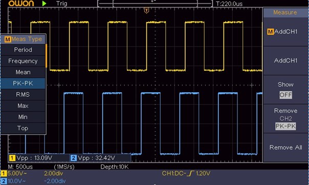
Figure 6-2 Waveform of Gain Measurement

Example 3: Capturing a Single Signal

It’s quite easy to use Digital Oscilloscope to capture non-periodic signal, such as a pulse and burr etc. But the common problem is how to set up a trigger if you have no knowledge of the signal? For example, if the pulse is the logic signal of a TTL level, the trigger level should be set to 2 volts and the trigger edge be set as the rising edge trigger. With various functions supported by our Oscilloscope, user can solve this problem by taking an easy approach. First to run your test using auto trigger to find out the closest trigger level and trigger type, this helps user to make few small adjustments to achieve a proper trigger level and mode. Here is how we achieve this.

The operation steps are as follows:

1. Set the probe menu attenuation coefficient to 10X and that of the switch in the probe to 10X
   (see “How to Set the Probe Attenuation Coefficient” on P11).
   
2. Adjust the Vertical
   Scale and Horizontal Scale knobs to set up a proper vertical and horizontal ranges for the signal to be observed.
   
3. Push the Acquire button to display the right menu.
   
4. In the right menu, select Acqu Mode as Peak Detect.
   
5. Push the Trigger Menu button to display the right
   menu.
   
6. In the right menu, select Type as Single.
   
7. In the right menu, select Single as Edge.
   
8. In the right menu, select Source as CH1.
   
9. In the right menu, press Next Page, select Coupling as DC.
   
10. In the right menu, select Slope as (rising).
    
11. Turn the Trigger Level knob and adjust the trigger level to the roughly 50% of the signal to be measured.
    
12. Check the Trigger State Indicator on the top of the screen, if it is not Ready, push down the Run/Stop button and start acquiring, wait for trigger to happen. If a signal reaches to the set trigger level, one sampling will be made and then displayed in the screen. By using this approach, a random pulse can be captured easily. For instance, if we want to find a burst burr of high amplitude, set the trigger level to a slightly higher value of the average signal level, push the Run/Stop button and wait a trigger. Once there is a burr occurring, the instrument will trigger automatically and record the waveform during the period around the trigger time. By turning the Horizontal Position knob in the horizontal control area in the panel, you can change the horizontal triggering position to obtain the negative delay, making an easy observation of the waveform before the burr occurs (see Figure 6-3).
    

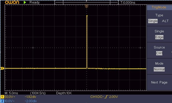
Figure 6-3 Capturing a Single Signal

Example 4: Analyze the Details of a Signal

Noise is very common inside most of the electronic signal. To find out what’s inside the noise and reduce the level of noise is very important function our oscilloscope is capable to offer.

Noise Analysis

The level of noise sometime indicates a failure of electronic circuit. The Peak Detect functions acts an important role to help you to find out the details of these noise. Here is how we do it:

1. Push the Acquire button to display the right
   menu.
   
2. In the right menu, select Acqu Mode as Peak Detect.
   

The signal displayed on the screen containing some noise, by turning on Peak Detect function and changing time base to slow down the incoming signal, any peaks or burr would be detected by the function (see Figure 6-4).

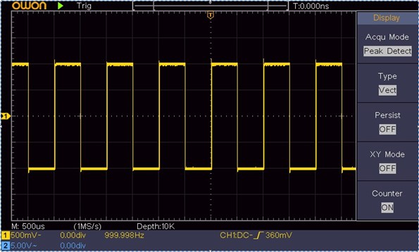
Figure 6-4 Signal with Noises

Separate Noises from the Signal

When focusing on signal itself, the important thing is to reduce the noise level as lower as possible, this would enable user to have more details about the signal. The Average function offered by our Oscilloscope can help you to achieve this.

Here are the steps for how to enable Average function.

1. Push the Acquire button to display the right menu.
   
2. In the right menu, select Acqu Mode as Average.
   
3. Turn the M knob and observe the waveform obtained from averaging the waveforms of different average number.
   

User would see a much reduced random noise level and make it easy to see more details of the signal itself. After applying Average, user can easily identify the burrs on the rising and falling edges of some part of the signal (see Figure 6-5).

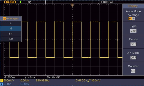
Figure 6-5 Reduce Noise level by using Average function

Example 5: Application of X-Y Function

Examine the Phase Difference between Signals of two Channels

Example: Test the phase change of the signal after it passes through a circuit network.

X-Y mode is a very useful when examining the Phase shift of two related signals. This example takes you step by step to check out the phase change of the signal after it passes a specified circuit. Input signal to the circuit and output signal from circuit are used as source signals.

For the examination of the input and output of the circuit in the form of X-Y coordinate graph, please operate according to the following steps:

1. Set the probe menu attenuation coefficient for 10X and that of the switch in the probe for 10X (see “How to Set the Probe Attenuation Coefficient” on P11).
   
2. Connect the probe of channel 1 to the input of the network and that of Channel 2 to the output of the network.
   
3. Push the Autoset button, with the oscilloscope turning on the signals of the two channels and displaying them in the screen.
   
4. Turn the Vertical
   Scale knob, making the amplitudes of two signals equal in the rough.
   
5. Push the Acquire button to display the right menu.
   
6. In the right menu, select XY Mode as ON. The oscilloscope will display the input and terminal characteristics of the network in the Lissajous graph form.
   
7. Turn the Vertical Scale and Vertical Position knobs, optimizing the waveform.
   
8. With the elliptical oscillogram method adopted, observe and calculate the phase difference (see Figure 6-6).
   

   
   

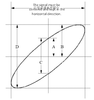
Figure 6-6 Lissajous Graph

Based on the expression sin (q) =A/B or C/D, thereinto, q is the phase difference angle, and the definitions of A, B, C, and D are shown as the graph above. As a result, the phase difference angle can be obtained, namely, q =± arcsin (A/B) or ± arcsin (C/D). If the principal axis of the ellipse is in the I and III quadrants, the determined phase difference angel should be in the I and IV quadrants, that is, in the range of (0 – π /2) or (3π / 2 – 2π). If the principal axis of the ellipse is in the II and IV quadrants, the determined phase difference angle is in the II and III quadrants, that is, within the range of (π / 2 – π) or (π – 3π /2).

Example 6: Video Signal Trigger

Observe the video circuit of a television, apply the video trigger and obtain the stable video output signal display.

Video Field Trigger

For the trigger in the video field, carry out operations according to the following steps:

1. Push the Trigger Menu button to display the right menu.
   
2. In the right menu, select Type as Single.
   
3. In the right menu, select Single as Video.
   
4. In the right menu, select Source as CH1.
   
5. In the right menu, select Modu as NTSC.
   
6. In the right menu, press Next Page, select Sync as Field.
   
7. Turn the Vertical Scale, Vertical Position and Horizontal Scale knobs to obtain a proper waveform display (see Figure 6-7).
   

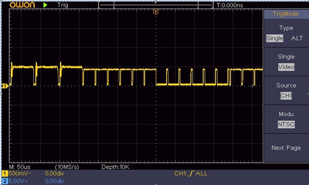
Figure 6-7 Waveform Captured from Video Field Trigger

7.Troubleshooting

7. Troubleshooting

• Oscilloscope is powered on but no Display.
  
  • Check whether the power connection is connected properly.
    
  • Restart the instrument after completing the checks above.
    
  • If the problem persists, please contact OWON and we will be under your service.
    
• After acquiring the signal, the waveform of the signal is not displayed in the screen.
  
  • Check whether the probe is properly connected to the signal connecting wire.
    
  • Check whether the signal connecting wire is correctly connected to the BNC (namely, the channel connector).
    
  • Check whether the probe is properly connected with the object to be measured.
    
  • Check whether there is any signal generated from the object to be measured (the trouble can be shot by the connection of the channel from which there is a signal generated with the channel in fault).
    
  • Make the signal acquisition operation again.
    
• The measured voltage amplitude value is 10 times or 1/10 of the actual value.
  

Look at the attenuation coefficient for the input channel and the attenuation ration of the probe, to make sure they are match
(see “How to Set the Probe Attenuation Coefficient” on P11).

• There is a waveform displayed, but it is not stable.
  
  • Check whether the Source item in the TRIG MODE menu is in conformity with the signal channel used in the practical application.
    
  • Check on the trigger Type item: The common signal chooses the Edge trigger mode for Type and the video signal the Video. If Alternate trigger is selected, both of the channel 1 and channel 2 trigger levels should be adjusted to the proper position. Only if a proper trigger mode is applied, the waveform can be displayed steadily.
    
• No Display Responses to the Push-down of Run/Stop.
  

  Check whether Normal or Signal is chosen for Polarity in the TRIG MODE menu and the trigger level exceeds the waveform range.
  

  If it is, make the trigger level is centered in the screen or set the trigger mode as Auto. In addition, with the Autoset button pressed, the setting above can be completed automatically.
  

• The displaying of waveform seems getting slow after increasing AVERAGE value in Acqu Mode (see “How to Set the Sampling/Display” on P27 ), or a longer duration is set in the Persist in Display (see “Persist” on P27).
  

  It’s normal as the Oscilloscope is working hard on many more data points.
  

8. Technical Specifications

Unless otherwise specified, the technical specifications applied are for the oscilloscope only, and Probes attenuation set as 10X. Only if the oscilloscope fulfills the following two conditions at first, these specification standards can be reached.

• This instrument should run for at least 30 minutes continuously under the specified operating temperature.
  
• If change of the operating temperature is up to or exceeds 5℃, do a “Self-calibration” procedure (see “How to Implement Self-calibration” on P12).
  

All specification standards can be fulfilled, except one(s) marked with the word “Typical”.

Trigger:

General Technical Specifications

Display

Output of the Probe Compensator

Power

Environment

Mechanical Specifications

Interval Period of Adjustment:

One year is recommended for the calibration interval period.

9.Appendix

9. Appendix

Appendix A: Enclosure

(The accessories subject to final delivery.)

Standard Accessories:

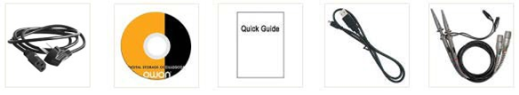
Power Cord     CD Rom     Quick Guide     USB Cable     Probe

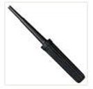
Probe Adjust

Options:

Soft Bag

Appendix B: General Care and Cleaning

General Care

Do not store or leave the instrument where the liquid crystal display will be exposed to direct sunlight for long periods of time.

Caution: To avoid any damage to the instrument or probe, do not exposed it to any sprays, liquids, or solvents.

Cleaning

Inspect the instrument and probes as often as operating conditions require. To clean the instrument exterior, perform the following steps:

1. Wipe the dust from the instrument and probe surface with a soft cloth. Do not make any scuffing on the transparent LCD protection screen when clean the LCD screen.
   

9.Appendix

1. Disconnect power before cleaning your Oscilloscope. Clean the instrument with a wet soft cloth not dripping water. It is recommended to scrub with soft detergent or fresh water. To avoid damage to the instrument or probe, do not use any corrosive chemical cleaning agent.
   

Warning: Before power on again for operation, it is required to confirm that

the instrument has already been dried completely, avoiding any electrical short circuit or bodily injury resulting form the moisture.

FNIRSl-10140 is a two in one oscilloscope and signal generator launched by FNIRSI, with comprehensive functions and high practiccibility. It is a cost-effective dual channel desktop oscilloscope for the maintenance industry and R&D industry. The oscilloscope has a real-time sampling rate of 1 GSa / s (giga samples), 100MHz* 2 analog bandwidth; complete trigger function (single time / normal / automatic), both for periodic analog signal and aperiodic digital signal can be used freely; built in DDS function signal generator and the industry’s original chopping output (@ 2.5VPP), all signal frequency step is 1Hz. support 14 kinds of standard function signal and a customizable chopping signal, chopping the output device intercepts part or the whole part of the complex signals measured by the oscilloscope as the output signal of the signal generator, which can store up to 1000 customized cut-off signals; the built-in high-voltage protection module can tolerate up to 400 continuous voltage, without worrying about the oscilloscope booming accident caused by the probe not moving to 10x gear. Large time base scrolling mode, which can monitor the slow level change; equipped with efficient one button auto, seIf-adaptive 25%, 50%, 75% trigger, which can display the measured waveform without complicated adjustment; the display is equipped with 7-inch 800 * 480 resolution high-definition LC screen; cursor measurement function, which can read the amplitude and frequency parameters manually without reading the background scale unit and quantity, and without conversion To get the peak and frequency directly; extremely convenient screen capture and waveform storage function, built-in 1GB storage space, cim store up to 1000 screen capture pictures + 1000 groups of waveform data, the storage process is simple and fast, save the current waveform, just a click to save the current data, very convenient; powerful waveform image manager, support thumbnail browsing, view, view details The functions of page turning, deleting and waveform enlarging, reducing and moving are convenient for secondary analysis. The fu    is equipped with USB interface, which can be connected with the computer to realize the sharing of its own screen capture pictures and the computer, which is convenient for secondary analysis; Lissajous graphic display function can be used to compare and judge the amplitude, frequency and phase of two groups of signals; FFT viewing function can roughly estimate the harmonic component of the signal; Lissajous graphic display function can be used to compare and judge the amplitude, frequency and phase of two groups of signals
!

1: When the two channels are used at the same time, the ground clamps of the two probes must be connected. It is strictly forbidden to connect the ground clamps of the two probes to different potentials, especially the different potential terminals of high-power equipment or 220 v. otherwise, the oscilloscope mother board will be bumped. Because the two channels are grounded together, connecting to different potentials will lead to the short circuit of the internal ground wire of the motherboard, and all oscilloscopes are same; 

2: The BNC input of oscilloscope can withstand 400 voltage at most. It is strictly forbidden to input more than 400 voltage in the position of 1x probe

 3: The original power supply must be used It is strictly forbidden to use the power supply or USB of other devices under the Otherwise, the motherboard ground wire may be short circuited during the test

4: 100 x
probe (such as ultrasonic welding machine, ultrasonic cleaning Machine etc.) or even 1000x probe (such as high-voltage end of high-frequency transformer, coil of induction cooker, etc.) must be used to measure high-frequency and high-voltage signal.

Solemnly remind

the bandwidth of 1x probe is 5MHz, and the bandwidth of 10x probe is 100MHz.

When the measurement frequency is higher than 5MHz, the switch on the probe handle needs to be moved to 10x, and the oscilloscope also needs to be set to 10x.

Otherwise, the signal will be greatly attenuated, which is the case with all oscilloscopes.

Because the probe line of the oscilloscope itself has a capacitance as high as 100 – 300pf, which is a big capacitance for high frequency signal! The signal has been greatly attenuated when it reaches the input end of the oscilloscope through the probe, and the equivalent bandwidth is 5 MHz. Therefore, in order to match the hundreds of PF of the probe line, the input end of the probe line will be attenuated 10 times (the switch is in the 10x gear), so that the hundreds of PF capacitor is just used for impedance matching. At this time, the bandwidth is 100MHz. Note that only

probes with 100MHz bandwidth or above can be used

Interface function indicator diagram

1: Run pause indicator

2: The trigger x position indication arrow indicates that this is the trigger x point

3: Background grid tick marks

4: Waveform data of channel 1

5: The baseline position of channel 1 indicates the arrow, that is, the position of OV potential

6: Waveform data of channel 2

7: The baseline position of channel 2 indicates the arrow, that is, the position of 0V potential

8: Horizontal time base control bar flag

9: Trigger the position of the X arrow relative to the system coordinate system

10: Horizontal time base refers to the length of time represented by a large grid in the horizontal direction, which is determined by the sampling rate. The larger the time base is, the slower the sampling rate is, and vice versa

11: Trigger status flag

12: Column 6 measurement parameters, press F6 to select measurement parameters freely

13: Column 5 measurement parameters, press FS to select measurement parameters freely

14: Column 4 measurement parameters, press F4 to select measurement parameters freely

15: Column 3 measurement parameters, press F3 to select measurement parameters freely

16: Column 2 measurement parameters, press F2 to select measurement parameters freely

17: Column 1 measurement parameters, press F1 to select measurement parameters freely

18: Channel 2 control bar sign

19: The input coupling mode of channel 1 has two options: DC and ac. DC means DC coupling and AC means AC coupling

20: Channel 1 probe magnification

21: Channel 1 control bar sign

22: vertical sensitivity of channel 1 refers to the voltage represented by a large grid in the vertical direction

23: Channel 1 baseline arrow position relative to the system coordinate system

24: movement speed of waveform operation, fast movement is used for coarse adjustment, and slow movement is used for fine adjustment

25: trigger voltage arrow position relative to the system coordinate system

26: trigger edge indicator, arrow up to rising edge trigger, arrow down to falling edge trigger

27: trigger mode indicator, divided into auto, single and normal; auto is automatic trigger, single is single trigger and normal is normal trigger

28: trigger control bar flag

29: trigger channel, divided into ch1 and CH2 options

Button function indication diagram

l pause button. Click. this button to pause sampling at any time

2: One key automatic adjustment button, click. this button, the system will automatically

identify the signal and set the system to the best parameters to display this waveform

3: Function menu button, click. hereto pop up the function menu

4: One click. screen capture button. Click. this button to take a screen capture of the

whole screen and save it to the interna! storage space automatically

5: One button save waveform button, click. this button will save all waveform data of

the two channels to the interna! storage space

6: Time cursor switch button, click. this button to turn on and off the cursor measurement

function

7: Press the voltage cursor switch keyto turn on and off the cursor measurement

function

8: System [right] navigation key

9: System navigation key

1 O: System [OK] navigation key

11: System navigation key

12: System [left] navigation key

13: Move speed button. Click. this button to switch between fast move and slow move

14: Channel 1 vertical position adjustment knob, rotate clockwise to move up, rotate

counterclockwise to move down

15: Channel 1 switch button. Click. this button to turn on or off the waveform display

of channel 1

16: Channel 1 control bar button. Click this button to pop up the control parameters

related to channel 1, which can be selected according to the navigation key or the

knob next to it

17: Channel 1 vertical sensitivity adjustment knob, clockwise vertical amplification,

counterclockwise vertical reduction

18: Channel 1 signal input port, the measurement range is O – 40V peak. to peak., pay

attention to the maximum tolerance of 400V peak. to peak. withstand voltage

19: Channel 2 vertical position adjustment knob, rotate clockwise to move up, rotate

counterclockwise to move down

20: Channel 2 switch button. Click this button to turn on or off the waveform display

of channel 2

21: Channel 2 control bar button. Click. this button to pop up the control parameters

related to channel 2, which can be selected according to the navigation key or the

knob next to it

22: Channel 2 vertical sensitivity adjustment knob, clockwise vertical amplification,

counterclockwise vertical reduction

23: Channel 2 signal input port. the measurement range is O – 40V peak. to peak., pay

attention to the maximum tolerance of 400V peak to peak withstand voltage

24: the system triggers the x position adjustment knob to move clockwise to the rig ht

and counterclockwise to the left

ZS: one key return to center button, after clicking this button, channel 1, channel 2

vertical position, trigger x horizontal position, trigger y vertical position will return to

center

Z6: the time base adjustment knob is rotated clockwise to reduce the time base, that

is, to enlarge the waveform horizontally, and counterclockwise to increase the time

base, that is, to reduce the waveform horizontally

Z7: DOS signal generator output

ZB: trigger voltage y position adjustment knob, rotate clockwise to move up, rotate

counterclockwise to move down

Z9: trigger mode switch button, divided into auto, single and normal

30: trigger edge switch button, divided into rising edge and falling edge

31: trigger channel switch button, divided into channel 1 and channel 2

32: 50% trigger button, click this button, the system will automatically set the current

trigger voltage to 25%, 50%, 75% according to the signal characteristics to trigger

33: the first column measurement parameter selection button, after the measurement

block diagram pops up, you can select according to the navigation key or the knob

next to it

34: the second column measurement parameter selection button, after the measurement

block diagram pops up, you can select according to the navigation key or the

knob next to it

35: the measurement parameter selection button in column 3, after the measurement

block diagram pops up, you can select according to the navigation key or the knob

next to it

36: the measurement parameter selection button in column 4, after the measurement

block diagram pops up, you can select according to the navigation key or the knob

beside it37: the measurement parameter selection button in column 5 pops up the

measurement block diagram, which can be selected according to the navigation key

or the knob beside it

38: the measurement parameter selection button in column 6, after the measurement

block diagram pops up, you can select according to the navigation key or the knob

beside it

39: signal generator control bar button, click this button will pop up the signal

generator parameter control bar, you can select according to the navigation key or

the knob next to it

40: next page of the control button on the next page of picture / waveform /

chopping Manager

41: picture l wave form l chopped wave manager next page control button [previous

page]

42: [delete] of the control button on the next page of picture l waveform l chopping

Manager

43: select a 11 of the control buttons on the next page of picture l waveform l chopping

Manager

44: [retum] of the control button on the next page of picture l waveform chopping

Manager

45: USB port for sharing screenshots

46: power switch, click to start or shut down operation

Operating instructions [oscilloscope part]

Open or close channel 1 / Channel 2:
click [ch1] / [CH2] to open or dose ch1 l CH2

Tum FFT on or off: click the [conf] button under ch1 or CH2, the parameter control bar

of channel 1 / Channel 2 will pop up, and then turn FFT on / off through the navigation

key

Setting input coupling mode:
click [conf] under ch1 or CH2 to pop up the parameter

control bar of channel 1 l Channel 2, and then switch DC l AC trough the navigation

key

Set the probe input ratio:
click [conf] under ch1 or CH2, the parameter control bar

of channel 1 l Channel 2 will pop up, and then switch to 1 x l 1 Ox / 1 OOx through the

navigation key

Scaling waveform: rotate the large knob at the bottom left corner of vertical frame

to scale the waveform of channel 1 vertically, and rotate the large knob at the bottom

right corner to scale the waveform of channel 2 vertically; rotate the large knob at the

bottom of horizontal frame to scale the waveform of channel 1 and channel 2

horizontally, clockwise to enlarge, counterclockwise to reduce

Moving waveform:
rotate the small knob in the upper left corner of vertical frame to

move the waveform of channel 1 vertically, and rotate the small knob in the upper

right corner to move the waveform of channel 2 vertically, which moves clockwise

upward and counterclockwise downward; rotate the small knob in the upper horizontal

frame to move the waveform of channel 1 and channel 2 horizontally, which moves

clockwise to the right and anticlockwise to the left In the process, you can click the

[slow] button to select coarse adjustment or fine adjustment

Adjust trigger voltage:
rotate the small knob under the trigger frame to adjust the

trigger voIta ge. In this process, you can click the [slow] button to select coarse adjustment

or fine adjustment. Pay attention to tum off the [automatic 50%] trigger in the

men u fi rst, otherwise the trigger voltage can not be adjusted

Set trigger edge:
click edge to switch rising edge l falling edge

Set auto trigger:
click mode to switch between auto l single l normal, where auto is

auto trigger

Set single trigger:
click mode to switch between auto l single l normal, where single

is single trigger

Set normal trigger: click mode to switch between auto l single l normal, where

normal is normal trigger

Pause display:
click the red [run l stop] button in the upper right corner to pause or

run

Automatic waveform adjustment: click the blue [auto] button in the upper right

corner to adjust automatically

Set the slow scan scrolling mode: rotate the big knob under the horizontal frame

counterclockwise. When the base reaches 1 OOms, the system will enter the slow scan

scrolling mode. 1 OOms – 50s belong to the time base of the scrolling mode

Time cursor measurement
click the [H cur] button to turn on the time cursor, and

then select the left and right light markings by the left and right keys of the navigation

key, and finally adjust them by the small knob in the upper left corner of the navigation

key, in which the light markings are moved to the right by clockwise rotation and

to the left by counterclockwise rotation

Voltage cursor measurement
click the [v cur] button to tum on the voltage cursor,

and then select the up and down light marking lines by the up and down keys of the

navigation key, and finally adjust them by the small knob in the upper left corner of

the navigation key, in which the light marking lines are moved upward by clockwise

rotation and downward by counterclockwise rotation

Set the parameters to be displayed:
click F1 – F6 to pop up the parameter measurement

control bar, and select the currently required parameters through the navigation

key or the nearby knob

Full screen capture:
click the [s pic] button to capture the current display. The

captured image is saved to the local disk in BMP format

s.va current waveform data: click the [s wav] button to save all waveform data of

the opened channel to the local disk

Adjust the screen brightness:
click the [menu] button, navigate to the [screen

brightness], press the OK key, and finally adjust the screen brightness through the

small knob in the upper left corner. 100 is the brightest and O is the darkest

Adjust the background grid brightness:
click the [menu] key, navigate to the [grid

brightness], press the OK key, and finally ad just t he grid brightness through the smal l

knob in the upper left corner. 100 is the brightest, and O is to turn off the grid display

Setting automatic 50% trigger all the time: click the [menu] key, navigate to

[automatic 50%], press the OK key, and then select [on] through the navigation key.

After setting, in the automatic trigger mode, each measurement system will automatically

set the trigger voltage to 25% / 50% / 75% of the peak to pea k value according

to the waveform characteristics

Horizontal baseline offset calibration:
when the probe has been pulled out, when

the left yellow l cyan indicator arrow and the Yellow l cyan horizontal baseline of

either channel are not in the same position, calibration is required; first pull out the

probe, then click the [menu] key, navigate to [baseline calibration], and then press the

OK key to calibrate the baseline

View the saved screen capture:
click [menu], navigate to [picture browse], and then

press the OK key to enter the picture thumbnail preview interface, which is the

thumbnail of the captured waveform. Select the thumbnail through the navigation

key, and then click [OKJ to view the screen capture of the waveform in full screen, with

(RET) return at the bottom, (SEL) All), (DEL), Oast), (next) the next control button can

be operated

View the saved waveform data:
click [menu] key, navigate to [waveform browse].

and then press the OK key to enter the waveform thumbnail preview interface, where

is the waveform thumbnail. Select the thumbnail through the navigation key, and

then click [OK] to view the waveform in full screen, with (REn retum at the bottom,

(SEL) All), (DEL), (last), (next) the next control button can be operated

Delete the saved waveform:
click the [menu] key, navigate to [waveform browse],

and then press the OK key to enter the waveform thumbnail preview interface, where

is the waveform thumbnail. Select the thumbnail through the navigation key, and

then click the [del] key at the bottom to delete the waveform, or click the key to delete

it in full screen view

Connect the computer to view the screen capture pictures:
click the [menu] button,

n¡¡vigate to the [USB share] through the navigation key, and then press the OK key to

open the USB share. Then connect the computer with the attached USB cable, and the

computer will pop up the removable disk or U-disk. Vau can find the screen capture

pictures saved in the disk in the computer. Note that you can’t repair them directly in

the disk Change the file name of the picture, otherwise the oscilloscope picture

manager will not be able to display the Picture

Operation instruction [signal generator part]

Switch the waveform type:
click the [Gen] button, the signal generator control

interface will pop up in the lower right corner of the screen, and then click the [OK]

button to switch the green selection box to the [waveform type] position, and then

click the [up] or [down] in the navigation key or the button in the upper left corner of

the navigation key to switch the waveform type

Adjust the waveform frequency:
click the [Gen] button, the sign¡il generator control

interface will pop up in the lower right corner of the screen, and then click the [OK]

button to switch the green selection box to the [frequency] position, and then click

the [left] or [right] in the navigation key to set the position cursor, that is, to set the

division to be adjusted. After confirming, press the [up] or [down] or the [up] button

in the upper left corner of the navigation key The knob can increase or decrease the

val u e of the current bit, thus changing the frequency

Adjust the duty cycle of square wave:
the duty cycle setting is only effective for

square wave. It can only be set when the waveform type is square wave. Other

waveforms h¡ive no concept of duty cycle. Click the [Gen] button, the signal generator

control interface will pop up in the lower right corner of the screen, and then click the

[OK] button to switch the green selection box to the [duty cycle] position, and then

rotate the navigation key in the upper left corner Vau can increase or decrease the

duty cycle with the knob of 1 % – 99%

Capture waveform:
Capture waveform output is to capture part or the whole part of

the current displayed waveform as the output of signal generator. The captured signa l

can be saved to the system, and up to 1000 groups of captured signals can be saved.

First. click the [menu] button, the function interface will pop up on the left side of the

screen, and then locate it to the capture output] position through the navigation key

and open it on the screen Two purple boundary lines will pop up. The waveform

within the two boundary lines is the waveform segment to be captured .The word

select indicates that the boundary line is the boundary line operated by the current

knob. You can switch and select the current operation line through the [left] and

[right] keys of the navigation key. After setting the boundilry line, you can go up to

the left through the navigation key When adjusting, you can click the [slow] key to set

coarse and fine adjustment; there is a word ‘channel 1 l Channel 2’ in the middle of

the two boundary lines, which means that the current captured signal is channel 1 l

Channel 2 signal, and you can select the channel through the [up] [down] of the

navigation key; the left boundary line is marked with voltage scale, which is used to

refer to the captured wave If you want to adjust the chopping level position, you can

adjust the offset by adjusting the Y position of the channel. For example, if you

captured a DC signal and adjust the DC waveform to+ 1V position, then the output

is + 1V voltage, and adjust to – 1V, then the output is – 1V voltage; If you want to

ildjust the sa m pi i ng ¡¡m plitude of chopped wave, you can adjust the verticil l sensitivity

of the channel to scale the waveform vertically. It is recommended to first amplify the

signal amplitude to the maximum, but not to cut the top, and then capture so that the

output signal will have enough sampling data, the output waveform distortion will be

smaller. and the resolution will be higher. If you only capture a very small signal, and

then capture it Output, and then through the oscilloscope meilsurement to enlarge it,

the waveform will appear a very serious ladder phenomenon, because the sampling

is insufficient, the effective signal is too little, just like the original image is very small,

but fon::ed to enlarge, the image is bound to be fuzzy; after all the parameters are

determined, click the [OKJ key, the cut-off will be saved to the system disk

Output the captured waveform as the signal generator:
first click the [Gen] button

to open the signa l generator interface, then click the [OK] button to switch the green

selection box to the [waveform type] position, and then click the [up] and [down] in

the navigation key to switch it to ‘self definition’, then click the [Gen] button to exit

the signal generator control interface, and then click the [ M ENU] button , the function

interface will pop up on the left side of the screen, and then navigate it to the [output

browsing] position and open it All saved captured signals will be listed on the screen,

and then the selection box will be moved to the desired signal position through the

navigation key. Click the [OKJ key, and the Yellow word ‘output’ will pop up in the

upper left corner of the w¡¡veform, which means that the current custom sign¡¡I

selection bit of the waveform Then click [menu] to exit, and the waveform output by

the signal generator is the captured signal. It should be noted that if the captured

waveform is a single cycle waveform, that is, there is only one cycle in the two bound

ary lines, then the output frequency of the signal generator is equal to the frequency

set by the signal generator. If the captured waveform frequency contains N cycles,

then the output frequency of the signal generator is n times of the set frequency, and

the trigger voltage should be adjusted to the minimum edge of the waveform In

other words, the intersection paint between the waveform and the trigger line is the

least:. otherwise the displayed frequency may be several times of the actual frequency,

because the calculated frequency of the oscilloscope is the frequency obtilined by

calculating the number of edges from the trigger line, so the wrong edge of the

positioning may also lead to frequency doubling

Analysis of common problems

1: Why can’t I turn on the machine after receiving it?

Answer: please check whether the power cord is connected to the oscilloscope and

whether the socket is powered. If all are correct. please replace a mobile phone

charging head and test it. If it is still unable to start. please contact customer service for replacement

2: Why Is there no waveform In the test, only one line on the screen Is still?

Answer: please check whether the pause has been pressed. If not. press the [auto]

button once. If not. it may be a problem that the signal source has no signal output.

or the probe line may be short circuited or open circuit. Please check whether the

probe and signal source are normal with multimeter

3: Why is the voltage value data 0?

Answer: please adjust the vertical sensitivity and time base (sampling rate), or press

[auto] screen to display at least a clear and complete periodic waveform, and the top

and bottom of the waveform should be displayed on the screen completely without

cutting the top. The voltage value data is correct at this time

4: Why is the frequency value data 0?

Answer: first. it is necessary to ensure that the trigger mode is auto automatic triggering.

if it is still O in auto mode, press [auto] button once. At least a clear and complete

periodic waveform is displayed on the screen, and the waveform should be triggered

(the green arrow indicates that the position is fixed between the wave shape and the

wave shape without shaking). The data of frequency value is correct

5: Why is the duty cycle 0?

Answer: first. it is necessary to ensure that the trigger mode is auto automatic triggering.

If it is still O in auto mode, it may be that the trigger is not adjusted to the

waveform. After the trigger line is adjusted to the waveform, the waveform will be

fixed. Moreover, the data of duty cycle will be correct only after at least one clear

periodic waveform is displayed on the screen

6: Why is AC coupling the same as DC coupling waveform?

Answer: if the input signal is a symmetrical AC signal (such as domestic 220V}, the AC

coupling or DC coupling waveform are the same. If it is an asymmetric AC signal or a

DC pulse signal, the waveform will move up and down when the coupling is switched

7: Why does the wavefonn run up and down when testing the signal, and can’t

see the wavefonn only see multiple online and offline beats?

Answer: set trigger mode to auto auto trigger, and then press [auto] button once. If it

is not solved, the clamp on the probe may not be grounded or the probe clamp end

is open circuit. Please check whether the probe is normal with multimeter

8: Why does the test wavefonn shake around and cannot be futed?

Answer: the trig g e r voltage needs to be adjusted, this is, the green arrow on the right

needs to adjust the green indicator to the top and bottom of the waveform. The

waveform is triggered and fixed, or the setting menu is entered to turn on “automatic

50%.’

9: Why can’t we capture sudden pulse waves or digital logic signals?

Answer: adjust the trigger mode to ‘Normal” or “Single’, then adjust the trigger

voltage and time base and vertical sensitivity, and finally touch the pause.

1 O: Why does trigger voltage regulation not respond?

Answer: click menu – Auto 50% to dose it

11: Why do you measure a battery or other DC voltage with out waveform?

Answer: battery voltage signal is stable DC signal, there is no curve waveform, in DC

coupled mode, and then adjust vertical sensitivity, there will be an upward or

downward offset straight line waveform, if it is AC coupling, no matter how to adjust.

there is no waveform.

12: why do we measure the 220V power frequency 50Hz wave?

Answer: if the oscilloscope displays SOHz low frequency signal, the sampling rate

needs to be very low to capture SOHz signal. If the sampling r11te is low, the oscilloscope

will enter the waiting, so it will show “card change’. All oscilloscopes in the

world will change their cards when measuring SOHz signals, not because the oscilloscope

itseIf is stuck

13: Why is the peak value of VPP more than 600 V and not 220V or 31 OV when

measuring the voltage wave form of the city power?

Answer: the city power 220V is a symmetrical AC signal, the positive peak voltage

(maximum value) is +310v, the negative peak voltage (minimum value) is -310v, sothe

peak value is 620V, the switching parameter is the effective value. At this time, it

is often said that the voltage of 220V, the effective value of the municipal voltage

fluctuates from 180 to 260V, so the peak VPP is in the range of 507-733v

14: Why is the measured voltage of 220V not a standard sine wave, there is

distortion?

Answer: in the municipal power grid, there are generally pollution, and there are more

high-order harmonic components. These harmonies will show a distorted sine wave

and normal phenomenon when superimposed on the sine wave. Generally, the shape

of the city electric wave is distorted, and it is irrelevant to the oscilloscope itself

15: Why is there a large offset between the baseline (OV) and the left arrow COV

indication} on the screen under no 5ignal input?

Answer: first pull out the probe, then click [menu] button, navigate to [baseline

calibration], then press OK, and wait for baseline calibration to complete, the baseline

and arrow coincide

16: Why is the signal voltage above 5MHz measured attenuated significantly, and

the bandwidth is only 5MHz?

Answer: when measuring 5MHz or more, it is necessary to move the probe to 10x

gear and the oscilloscope should be set to 1 Ox input mode, because the probe line of

the oscilloscope has a capacitance of up to 100-300pf, which is a big capacitance for

high frequency signal! The signal has been greatly attenuated when it reaches the

input end of the oscilloscope through the probe, and the equivalent bandwidth is

SMHz. So in order to match hundreds of PF of probe line, it will be decayed 1 O times

at the input end of probe line (switch is in 10x), so that these hundreds of PF capacitors

are just used for impedance matching. At this time, the bandwidth is 100MHz.

Note that only the supporting 100 MHz probe can be used

Test methods of common circuits

Battery or DC voltage measurement

Gear selection: the battery voltage is generally below 40V, other DC voltage is

uncertain, so it is necessary to adjust the gear according to the actual situation. if it

is higher than 40V (both probe and oscilloscope are set to the same gear)

1: Firstly, the oscilloscope is set to auto trigger mode (auto trigger mode is default

after startup), and auto trigger mode is used to test the cycle signal (DC voltage

belongs to the periodic signal)

2: The oscilloscope probe multiplier is set to the corresponding gear (default is 1x

after startup)

3: Oscilloscope coupling mode is set to DC coupling mode

4: Insert the probe and move the switch on the probe handle to the corresponding

gear

5: Make sure the battery is powered or the DC voltage is voltage output

6: Connect the probe clip to the negative battery or the negative DC electrode, and

the probe to the battery or DC positive pole

7: Press [auto] once, the DC electrical signal will be displayed. Then, look at the

parameter of average value. Note that battery voltage or other DC voltage belong to

DC signal, and there is no curve waveform, only a line with up and down offset and

the peak value and frequency of this signal are O

Crystal vibration measurement

Gear selection: crystal oscillator is easy to stop oscillation after encountering capacitance.

input capacitance of 1x probe is up to 100-300pf, 10x gear is about 10-30pf,

and it is easy to stop vibration in 1x gear, so it is necessary to set 1 Ox gear, that is, both

probe and oscilloscope should be switched to 10x gear (probe and oscilloscope are

set to 10x gear)

1: Firstly, the oscilloscope is set to auto trigger mode (auto trigger mode is default

after startup), and auto trigger mode is used to test the periodic signal (the sine signa l

of crystal resonance belongs to the periodic signal

2: The oscilloscope probe multiplier is set to 10x (default is in the 1x gear after

startup)

3: Oscilloscope coupling mode is set to AC coupling mode

4: insert the probe and move the switch on the probe handle to 10x

5: Make sure the crystal board is powered on and running

6: Connect the probe clip to the ground wire of the crystal oscillator board (negative

pole of power supply), pull the probe cap out, and inside it is the needle tip, which

contacts one of the pins of the crystal oscillator

7: Press the [auto] button once to display the waveform of the crystal vibration tested.

If the waveform after automatic adjustment is too small or too large, the waveform

size can be adjusted manually by knob

PWM signal measurement of MOS tube or IGBT

Gear selection: the PWM signal voltage of direct drive MOS tube or IGBT is generally

within 10v-20v, the control signal of PWM front stage is also generally within 3-20v,

and the maximum test of 40V in the 1x gear is enough. Therefore, it is enough to

test the PWM signal with the 1x gear (both probe and oscilloscope are set to the 1x

gear).

1: Firstly, the oscilloscope is set to auto trigger mode (auto trigger mode is default

after startup), and auto trigger mode is used to test cycle signal (PWM belongs to

cycle signal

2: The oscilloscope probe multiplier is set to the 1x gear (default is 1x gear after

startup)

3: Oscilloscope coupling mode is set to DC coupling mode

4: insert the probe and move the switch on the probe handle to the 1x position

5: Make sure that the PWM main board has PWM signal output at this time

6: Clip the probe to the S-pole of the MOS tube and the probe to the g-pole of the

MOS tube

7: Press the [auto] button once to display the measured PWM waveform. if the

waveform after automatic adjustment is too small or too large, the waveform size can

be adjusted manually by knob

Signal generator output measurement

Gear selection: the output voltage of signal generator is within 30V, and the maximum

test value of 1x gear is 40V, so the output of test signal generator is in the 1x gear

(probe and oscilloscope are set to be 1 x gear).

1: Firstly, the oscilloscope is set to auto trigger mode (the default mode is auto trigger

mode after startup), and auto trigger mode is used to test the periodic signal (the

signal output by the signal generator belongs to the periodic signaO

2: The oscilloscope probe multiplier is set to the 1x gear (default is 1x gear after

startup)

3: Oscilloscope coupling mode is set to DC coupling mode

4: insert the probe and move the switch on the probe handle to the 1x position

5: Make sure the signal generator is on and is outputting the signal

6: Connect the probe clip to the black clip of the signal generator output line, and the

probe to the red output line of the signa l generator

7: Press the [auto] button once, the waveform output by the generator will be

displayed. If the waveform after automatic adjustment is too small or too large, the

waveform size can be adjusted manually by knob

Measurement of domestic electricity at 220V or 110V

Gear selection: first, you need to buy 1 OOx probe; household electric power generally

180-260V, peak peak voltage is 507-733v, the maximum measurement of 1x is 40V,

the highest val u e of 1 Ox is 400V, 1 OOx is 4000V, and the default standard probe is 1 Ox

high voltage probe, and the peak value of 400V can only be measured. Therefore,

1 OOx probe shall be provided by itseIf, and then set to 1 OOx gear, that is, both probe

and oscilloscope shall be switched to 1 OOx gear

1: Firstly, the oscilloscope is set to auto trigger mode (auto trigger mode is default

after startup), and auto trigger mode is used to test the cycle signal (50Hz of household

electric power belongs to the periodic signal)

2: The oscilloscope probe multiplier is set to 100x (default is in the 1x gear after

startup)

3: Oscilloscope coupling mode is set to AC coupling mode

4: insert the probe and move the switch on the probe handle to 100X

5: Ensure that the tested end has a home power output

6: Connect the probe clip and probe to 2 wires of household electric power without

distinguishing the positive and negative pales

7: Press the [auto] button once to display the waveform of the household electric

power. If the waveform after automatic adjustment is too small or too large, the

waveform size can be adjusted manually by the knob

Power ripple measurement

Gear selection: if the output voltage of power supply is below 40V, it is set to the 1x

gear (both probe and oscilloscope are set to 1x gear), and 10x gear (both probe and

oscilloscope are set to the same gear if they are 40-400v}

1: Firstly, the oscilloscope is set to auto trigger mode (auto trigger mode is default

after startup), and auto trigger mode is used to test the cycle signal (DC voltage

belongs to the periodic signal)

2: The oscilloscope probe multiplier is set to the corresponding gear (default is 1x

after startup)

3: The oscilloscope coupling mode is set to AC coupling mode, note that AC AC

coupling mode

4: Insert the probe and move the switch on the probe handle to the corresponding

gear

5: Make sure the power is powered on and voltage output is available

6: Connect the probe clip to the negative extreme of the power output, and the probe

is connected to the positive extreme of the power output, and wait for about 3

seconds. When the yellow line and the left yellow arrow position are in the same

position, wait until the position is in the same position

7: Press the [auto] button once, and the power ripple will be displayed

Inverter output measurement

Gear selection: the output voltage of inverter is similar to that of household electricity,

with peak voltage above 500V, the highest measurement of 40V in 1X, 400V in

1 Ox and 4000V in 1 OOx gear. The default standard probe is 1 Ox hi g h voltage probe,

and the peak value of 400V can only be measured at the highest. Therefore, 100x

probe shall be provided by itself, and then set to 1 OOx gear, that is, both probe and

oscilloscope shall be switched to 1 OOx gear

1: Firstly, the oscilloscope is set to auto trigger mode (the default mode is auto trigger

mode after startup), and auto trigger mode is used to test the periodic signal (the

signal output by the inverter belongs to the pericolic signal

2: The oscilloscope probe multiplier is set to 100x (default is in the 1x gear after

startup)

3: Oscilloscope coupling mode is set to DC coupling mode

4: Insert the probe and move the switch on the probe handle to 100X

5: Ensure inverter is powered on and voltage output is available

6: Connect the probe clamp and probe to the output end of the inverter without

distinguishing the positive and negative poles

7: Press the [auto] button once to display the waveform of the inverter. If the

waveform after automatic adjustment is too small or too large, the waveform size can

be adjusted manually by knob

Measurement of power amplifier or audio signal

Gear selection: the output voltage of power amplifier is generally below 40V, and the

maximum test of 40V in the 1x gear is enough {both probe and oscilloscope are set

to the 1 x gear).

1: First set the oscilloscope to auto trigger mode {the default is auto trig ge r mode

after startup)

2: The oscilloscope probe multiplier is set to the 1x gear (default is 1x gear after

startup)

3: Oscilloscope coupling mode is set to AC coupling mode

4: Insert the probe and move the switch on the probe handle to the 1x position

5: Ensure that the amplifier is on and is outputting audio signals

6: Connect the probe clip and probe to the output end of 2 lines of the amplifier

without distinguishing the positive and negative poles

7: Press the [auto] button once to display the waveform of the inverter. If the

waveform after automatic adjustment is too small or too large, the waveform size can

be adjusted manually by knob

Measurement of vehicle communication signal J bus signal

Gear selection: the communication signal of automobile is generally lower than 20V,

and the maximum test for 1x gear is 40V, so it is enough to test the vehicle communication

signal with the 1x gear (both probe and oscilloscope are set to the 1x

gear).

1: Firstly, the oscilloscope is set to normal trigger mode (auto trigger mode is

default after startup). Normal trigger mode is specially used to measure the non

periodic digital signal. If Auto trigger mode is used, it is impossible to grasp the non

periodic signal

2: The oscilloscope probe multiplier is set to the 1x gear (default is 1x after startup)

3: Oscilloscope coupling mode is set to AC coupling mode

4: Insert the probe and move the switch on the probe handle to the 1x position

5: Connect the probe clip and probe to two signal lines of communication line,

regardless of positive and negative. If there are multiple signal lines, you need to

judge the signal line in advance, or try to select two of them for testing several times

6: Make sure that there is a communication signal on the communication line at this

time

7: Adjust the vertical sensitivity to 50mV

8: Time base to 20us

9: Press [50%] once

10: When there is communication signal on the communication line, the oscilloscope

will capture and display it on the screen. if it can not be captured, it is necessary to try

to ad just the time base (1 ms-100ms) and trigger voyage {green arrow) for multiple

times

Infrared remote receiver measurement

Gear selection: the infrared remote control signal is generally 3-5v, and the maximum

test for 1x gear is 40V, so it is enough to test the vehicle communication signal signa l

with the 1x gear {both the probe and oscilloscope are set to the 1x gear).

1: Firstly, the oscilloscope is set to normal trigger mode {auto trigger mode is

default after startup). Normal trigger mode is specially used to measure the non

periodic digital signal. If the auto trigger mode is not able to grasp the non periodic

signal, the infrared remote control signal belongs to the non periodic digital coding

signal

2: The oscilloscope probe multiplier is set to the 1x gear (default is 1x after startup)

3: Oscilloscope coupling mode is set to DC coupling mode

4: Insert the probe and move the switch on the probe handle to the 1x position

5: Connect the probe clip to the ground end (negative) of the infrared receiver board,

and the probe to the data pin of the infrared receiver

6: Adjust the vertical sensitivity to 500mv

7: Time base to 20us

8: Tum the trigger red arrow position to the left yellow arrow position and approximately

1 large grid distance

9: At this time, the infrared receive hair signal is sent by remate control, and the

waveform will appear on the oscilloscope

Measurement of amplification circuit with sensors (temperature, humidity,

pressure, hall, etc.)

Gear selection: generally, the sensor signal is relatively weak, about a few millivolts.

This small signal cannot be detected directly by oscilloscope. There is signal amplification

part on the main board of this sensor. When the output end of the amplifier is

found, the oscilloscope can measure the signal after being enlarged. It can be used in

the 1x gear (both probe and oscilloscope are set to the 1x gear)

1: First set the oscilloscope to auto trigger mode (the default is auto trigger mode

after startup)

2: The oscilloscope probe multipliers is set to the 1x gear (default is 1x after startup)

3: Oscilloscope coupling mode is set to DC coupling mode

4: Insert the probe and move the switch on the probe handle to the 1x position

5: Connect the probe clip to the ground end of the sensor motherboard (negative

power supply), find the output end of the amplification part, and connect the probe

to the output end

6: Adjust the vertical sensitivity to 50 mV

7: Adjust the time base to 500ms and enter the slow scan mode of large time base

8: Move baseline to bottom

9: If the signal line appears at the top, the vertical sensitivity shall be reduced, which

is 100mV, 200mV, 500mv, etc. in turn, when the updated signal on the right starts not

at the top (generally the best in the middle of the upper and lower part), the signal

received by the sensor can be detected.